PySINDy from the ground up: predator-prey equations from data

The problem: which equations made these populations?

Here are two time series from a predator-prey system: prey \(x\) and predators \(y\), in thousands, counted 200 times over 24 years. The prey swing between 0.66 and 8.22 thousand, the predators between 0.165 and 1.125 thousand, in cycles of about 8.9 years. Which differential equations produced them? SINDy (sparse identification of nonlinear dynamics), in Python the PySINDy package, writes each rate of change, \(\dot x = dx/dt\) and \(\dot y\), as a sum over a library of candidate terms, here the six products of \(x\) and \(y\) up to degree two: \(1, x, y, x^2, xy, y^2\). Sparse regression then keeps the few terms the data need and sets the others to zero.

The data come from the Lotka-Volterra model with the rates of Draw a phase portrait of a two-variable ODE system,

\[\dot x = \alpha x - \beta xy, \qquad \dot y = \delta xy - \gamma y ,\]

with \(\alpha = 1.0\) and \(\gamma = 0.6\) per year, \(\beta = 2.0\) and \(\delta = 0.2\) per thousand per year. So the right answer is known: four nonzero coefficients out of twelve. The linear counterpart, a model fitted to a measured input and output, is System identification.

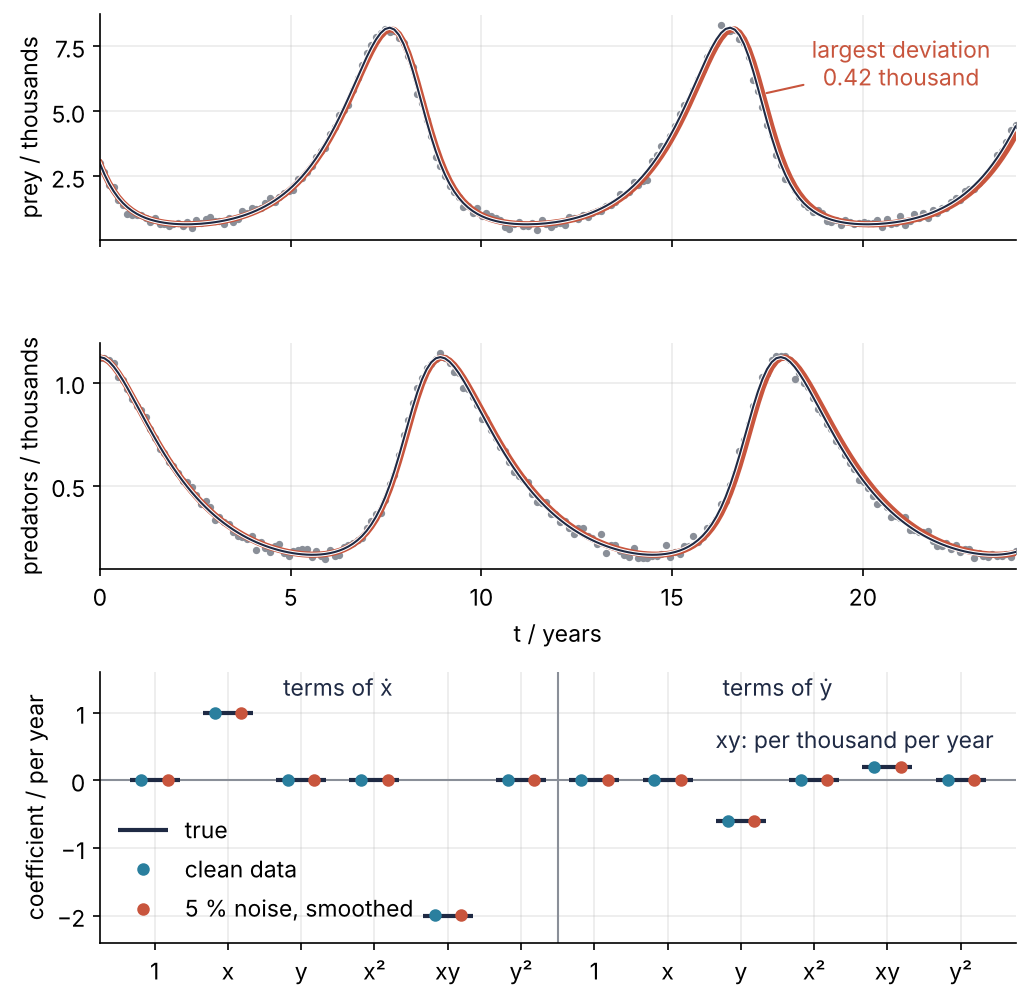
Prey and predators in thousands over 24 years: data with 5 % noise as gray dots, the clean trajectory a thin dark line, the PySINDy model red, lagging slightly after year 16, largest prey deviation 0.42 thousand. Below: the twelve coefficients, true values as bars, clean and noisy fits as dots.

This is where we end up. From data with 5 % noise, PySINDy returns the four true terms and nothing else, and the identified model, simulated from the first sample, stays within 0.42 thousand prey of the clean trajectory over 24 years. Over 20 noise realizations it finds exactly those four terms in 17 at 2 % noise, in 15 at 5 % with smoothing, and at 20 % in one at most.

Setup

import warnings
import numpy as np
import matplotlib.pyplot as plt
from scipy.integrate import solve_ivp
import pysindy as ps

plt.rcParams.update({
    "figure.figsize": (7, 3.6), "figure.dpi": 110,
    "axes.spines.top": False, "axes.spines.right": False,
    "axes.grid": True, "grid.alpha": 0.25,
    "font.size": 11, "lines.linewidth": 1.8,
})
INK, ACCENT, SECOND, MUTED = "#1f2a44", "#c8553d", "#2a7f9e", "#8a8f98"

alpha, gamma = 1.0, 0.6        # prey growth, predator death; per year
beta, delta = 2.0, 0.2         # predation, predator gain; per thousand per year

def f(t, z):
    x, y = z
    return np.array([alpha * x - beta * x * y, delta * x * y - gamma * y])

t = np.linspace(0, 24, 200)                                    # years
X = solve_ivp(f, (0, 24), [3, 1.125], t_eval=t, rtol=1e-10, atol=1e-12).y.T
X_dot_true = f(0, X.T).T
XI_TRUE = np.array([[0, alpha, 0, 0, -beta, 0],                # terms 1, x, y, x^2, xy, y^2
                    [0, 0, -gamma, 0, delta, 0]])

rng = np.random.default_rng(0)
X_noisy = X + 0.05 * X.std(axis=0) * rng.standard_normal(X.shape)

print(f"{len(t)} samples, spacing {t[1] - t[0]:.3f} years")
print(f"x from {X[:, 0].min():.2f} to {X[:, 0].max():.2f}, y from {X[:, 1].min():.3f} to {X[:, 1].max():.3f} thousand")

200 samples, spacing 0.121 years
x from 0.66 to 8.22, y from 0.165 to 1.125 thousand

Step 1: Fit a first model and name its three parts

PySINDy wants one row per time and one column per variable, the transpose of sol.y, so X has shape (200, 2). Fit the default model to the clean data. In PySINDy 2.x the variable names go to fit:

model = ps.SINDy()
model.fit(X, t=t, feature_names=["x", "y"])
model.print()

(x)' =  0.996 x + -1.993 x y
(y)' = -0.598 y +  0.199 x y

The right four terms, each about 0.4 % too small, and the other eight coefficients exactly zero. x y is the product, and + -1.993 is how PySINDy writes a minus. A model has three parts, each a choice.

Derivatives. PySINDy has samples, not rates, so it estimates the rate at each sample from the slope between its two neighbors, \((x_{i+1} - x_{i-1})/(2\Delta t)\). This is a finite difference, ps.FiniteDifference().

Library. Each candidate term is evaluated at every sample, which gives a table \(\Theta(X)\) of 200 rows and six columns, ps.PolynomialLibrary(degree=2).

Optimizer. It looks for the coefficients that make the library's columns add up to the estimated rates, \(\dot X \approx \Theta(X)\,\Xi\), by least squares, with \(\Xi\) the twelve coefficients, one column per equation. Coefficients smaller than a threshold, 0.1 by default, are set to zero, the fit is redone with the surviving terms, and this repeats until nothing changes. That is sequentially thresholded least squares, ps.STLSQ. Here are the parts plugged in explicitly:

model = ps.SINDy(feature_library=ps.PolynomialLibrary(degree=2),
                 optimizer=ps.STLSQ(threshold=0.1),
                 differentiation_method=ps.FiniteDifference(order=2))
model.fit(X, t=t, feature_names=["x", "y"])

print(model.get_feature_names())
with np.printoptions(precision=3, suppress=True):
    print(model.coefficients())
    print(XI_TRUE)
print(f"score R² = {model.score(X, t=t):.5f}")

['1', 'x', 'y', 'x^2', 'x y', 'y^2']
[[ 0.     0.996  0.     0.    -1.993  0.   ]
 [ 0.     0.    -0.598  0.     0.199  0.   ]]
[[ 0.   1.   0.   0.  -2.   0. ]
 [ 0.   0.  -0.6  0.   0.2  0. ]]
score R² = 0.99998

coefficients() prints \(\Xi\) transposed, one row per equation in the order of the feature names, so it lines up with XI_TRUE. The score is R² of the rates the model predicts against the rates estimated from the data. It is near 1 here; Pitfall 2 shows what it misses.

Step 2: Choose the candidate terms from the mechanism

For a system whose equations you do not know, the library is your hypothesis. Write down what each process does to the rates. Births and deaths in proportion to a population give terms in \(x\) and \(y\). Encounters, at a rate proportional to both populations, give the product \(xy\). Crowding of the prey would give \(x^2\). Take the smallest library that contains every term the mechanism allows, here polynomials up to degree two. A process that is not a polynomial, a predator that saturates as \(x/(1+x)\), needs a custom term (see the variations). Leave out the interaction, and this is what happens:

model_1 = ps.SINDy(feature_library=ps.PolynomialLibrary(degree=1))
with warnings.catch_warnings(record=True) as caught:
    warnings.simplefilter("always")
    model_1.fit(X, t=t, feature_names=["x", "y"])
model_1.print()
print("warning:", caught[0].message)
print(f"score R² = {model_1.score(X, t=t):.3f}")

(x)' =  2.756 1 + -5.479 y
(y)' =  0.000
warning: Sparsity parameter is too big (0.1) and eliminated all coefficients
score R² = 0.354

The "1" in the printout is the constant term. A library without \(xy\) cannot write the interaction, so the prey equation becomes a constant minus predators and the predator equation is emptied. A score of 0.354 says the model is wrong. The opposite mistake, more terms than one record can tell apart, is Pitfall 2.

Step 3: Choose the sparsity threshold

The threshold decides which terms survive. Sweep it and count them. The last three lines fit the predator rates with \(y\) alone; that number explains the cliff below:

print("threshold  terms  score")
for threshold in [0.001, 0.003, 0.01, 0.03, 0.1, 0.19, 0.21, 0.3, 1.0]:
    with warnings.catch_warnings(record=True) as caught:
        warnings.simplefilter("always")
        m = ps.SINDy(optimizer=ps.STLSQ(threshold=threshold)).fit(X, t=t)
    note = "  an equation emptied" if caught else ""
    print(f"{threshold:9.3f}  {np.count_nonzero(m.coefficients()):5d}  {m.score(X, t=t):6.3f}{note}")

X_dot = ps.FiniteDifference()(X, t)
y = X[:, 1]
print(f"best coefficient of y alone in the predator equation: {y @ X_dot[:, 1] / (y @ y):.3f}")

threshold  terms  score
    0.001     12   1.000
    0.003      9   1.000
    0.010      6   1.000
    0.030      4   1.000
    0.100      4   1.000
    0.190      4   1.000
    0.210      2   0.488  an equation emptied
    0.300      2   0.488  an equation emptied
    1.000      0  -0.012  an equation emptied
best coefficient of y alone in the predator equation: -0.073

Below 0.03 spurious terms survive, all twelve at 0.001. From 0.03 to 0.19 the count sits at four, the true model, and up to 0.19 the score reads 1.000 whatever the count. Just above 0.2 the count falls off a cliff. At 0.21 the first fit, with all six terms, finds \(xy\) in the predator equation near its true 0.2, below the threshold, so it goes. The refit has only \(y\) left to explain \(\dot y\), and over whole cycles the predators rise as much as they fall, so its best coefficient, the last line, is \(-0.073\). It is below the threshold too, and the predator equation empties. Take the threshold from the middle of the last plateau before the cliff, below the smallest coefficient you expect, and never from the score alone.

Step 4: Check the model by simulating it

A model of the rates is only as good as the trajectory it produces. simulate integrates the identified equations from a starting state with solve_ivp:

def deviation(X_a, X_b):
    d = np.abs(X_a - X_b).max(axis=0)
    return f"largest deviation: prey {d[0]:.3f}, predators {d[1]:.3f} thousand"

X_sim = model.simulate(X[0], t)
print(deviation(X_sim, X))

largest deviation: prey 0.329, predators 0.039 thousand

The simulation drifts to 0.33 thousand prey off the data over 24 years. The deviation grows with time, because a rate 0.4 % too small lengthens the period and the phase slides. The cause is the derivative estimate of Step 1. Its error shrinks with the square of the spacing: halve \(\Delta t\) and the error drops to a quarter. That is order 2, the default. ps.FiniteDifference(order=4) uses two neighbors on each side, and its error shrinks with the fourth power:

model_4 = ps.SINDy(differentiation_method=ps.FiniteDifference(order=4))
model_4.fit(X, t=t, feature_names=["x", "y"])
model_4.print(precision=4)
print(deviation(model_4.simulate(X[0], t), X))

(x)' =  1.0000 x + -1.9999 x y
(y)' = -0.6000 y +  0.2000 x y
largest deviation: prey 0.003, predators 0.000 thousand

Four digits right, and the simulation a hundred times closer. On clean data the derivative estimate sets the accuracy, and the derivative estimate is what noise attacks.

Step 5: Add noise, and smooth before differentiating

Estimate the rates of the 5 % record with plain and with smoothed finite differences, and compare each with the true rates:

fd = ps.FiniteDifference()
sfd = ps.SmoothedFiniteDifference()
for name, diff in [("finite differences", fd), ("smoothed", sfd)]:
    error = diff(X_noisy, t) - X_dot_true
    rel = np.sqrt((error**2).mean(axis=0)) / X_dot_true.std(axis=0)
    print(f"{name:18s}  rms error / std of rate:  x {rel[0]:.2f}   y {rel[1]:.2f}")

finite differences  rms error / std of rate:  x 0.32   y 0.39
smoothed            rms error / std of rate:  x 0.10   y 0.09

The 5 % noise in the data becomes 32 and 39 % in the rates. The difference of two neighbors keeps the full noise of both samples but only a sliver of the signal, which changes little in \(2\Delta t = 0.24\) years.

SmoothedFiniteDifference first smooths the data, by Savitzky-Golay (scipy.signal.savgol_filter): in a window around each sample it fits a low-degree polynomial by least squares and replaces the sample by the polynomial's value. The defaults, 11 samples (1.2 years) and a cubic, follow the population cycles, much wider than the window, but not the scatter from one sample to the next. That cuts the error to 10 and 9 %.

first = t <= 9
fig, ax = plt.subplots(figsize=(7, 3.2))
ax.plot(t[first], fd(X_noisy, t)[first, 1], "o-", color=MUTED, ms=3, lw=0.8)
ax.plot(t[first], X_dot_true[first, 1], color=INK)
ax.plot(t[first], sfd(X_noisy, t)[first, 1], color=ACCENT)
ax.text(4.6, 0.28, "finite differences", ha="center", color=MUTED)
ax.text(1.6, -0.45, "true", color=INK)
ax.text(7.45, 0.6, "smoothed", ha="right", color=ACCENT)
ax.set(xlabel="t / years", ylabel="ẏ / thousand per year", xlim=(0, 9))
plt.show()

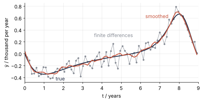
Rate of change of the predators over the first nine years, in thousand per year. Finite differences of data with 5 % noise miss the true curve by up to a fifth of its swing; the smoothed estimate follows the true curve closely.

The gray points miss the true curve by up to 0.22 thousand per year, a fifth of its swing; the smoothed curve lies on the true one. Fit both:

for name, diff in [("finite differences", ps.FiniteDifference()), ("smoothed", ps.SmoothedFiniteDifference())]:
    m = ps.SINDy(differentiation_method=diff)
    m.fit(X_noisy, t=t, feature_names=["x", "y"])
    print(name)
    m.print()
    print(deviation(m.simulate(X_noisy[0], t), X), "\n")
model_noisy = m                                               # the smoothed fit, the last of the loop

finite differences
(x)' =  0.983 x + -1.973 x y
(y)' = -0.597 y +  0.201 x y
largest deviation: prey 0.972, predators 0.125 thousand 

smoothed
(x)' =  0.995 x + -1.991 x y
(y)' = -0.597 y +  0.200 x y
largest deviation: prey 0.418, predators 0.055 thousand

Both keep the right terms here. In the prey equation the smoothed coefficients are three times closer to the truth, and the simulation, started from the first noisy sample, strays 0.42 thousand prey from the clean trajectory instead of 0.97.

Step 6: Find how much noise the method tolerates

One noisy record says little: another draw of the noise might lose a term. Repeat with 20 realizations at each of six noise levels and count the runs whose nonzero coefficients sit exactly where those of XI_TRUE do:

levels = [0, 0.01, 0.02, 0.05, 0.10, 0.20]
print("noise level            " + "".join(f"{level:6.0%}" for level in levels))
for name, make in [("finite differences", ps.FiniteDifference), ("smoothed", ps.SmoothedFiniteDifference)]:
    counts = []
    for i, level in enumerate(levels):
        hits = 0
        for trial in range(20):
            noise = np.random.default_rng([i, trial]).standard_normal(X.shape)
            with warnings.catch_warnings():
                warnings.simplefilter("ignore", UserWarning)     # an emptied equation is counted as a miss anyway
                m = ps.SINDy(differentiation_method=make()).fit(X + level * X.std(axis=0) * noise, t=t)
            hits += np.array_equal(m.coefficients() != 0, XI_TRUE != 0)
        counts.append(hits)
    print(f"{name:18s} of 20 " + "".join(f"{c:6d}" for c in counts))

noise level                0%    1%    2%    5%   10%   20%
finite differences of 20     20    20    17     6     4     1
smoothed           of 20     20    20    17    15    12     0

Both are reliable up to 1 % and find the model in 17 of 20 runs at 2 %. At 5 % smoothing wins, 15 against 6. At 10 % smoothing still finds it in 12 runs and plain differences in 4; at 20 % neither works, with 1 and 0. With one record of 200 samples, the derivative estimate fails first. Above a few percent of noise you need more data or a method that avoids differentiating, not a different threshold.

Your own record has neither XI_TRUE nor a clean trajectory, so judge it against itself. The scatter of the raw samples about the smoothed ones, sfd.smoothed_x_, estimates the noise, and a right model simulates within a few such widths of the data:

scatter = np.sqrt(((sfd.smoothed_x_ - X_noisy)**2).mean(axis=0))   # the noise, estimated from the data
print(f"scatter: prey {scatter[0]:.3f} thousand (noise added: {0.05 * X[:, 0].std():.3f})\n")
print("threshold  terms  rms(simulation - data) / scatter")
for threshold in [0.01, 0.03, 0.1, 0.15, 0.21]:
    with warnings.catch_warnings():
        warnings.simplefilter("ignore", UserWarning)
        m = ps.SINDy(optimizer=ps.STLSQ(threshold=threshold),
                     differentiation_method=ps.SmoothedFiniteDifference()).fit(X_noisy, t=t)
    r = np.sqrt(((m.simulate(X_noisy[0], t) - X_noisy)**2).mean(axis=0)) / scatter
    print(f"{threshold:9.2f}  {np.count_nonzero(m.coefficients()):5d}  prey {r[0]:4.1f}  predators {r[1]:4.1f}")

scatter: prey 0.098 thousand (noise added: 0.115)

threshold  terms  rms(simulation - data) / scatter
     0.01     10  prey  2.5  predators  1.8
     0.03      7  prey  1.2  predators  1.1
     0.10      4  prey  1.9  predators  1.6
     0.15      4  prey  1.9  predators  1.6
     0.21      2  prey 35.0  predators 47.6

The scatter is close to the noise added, and the count falls in stairs to the cliff, where the simulation leaves the data by 35 and 48 widths. Before it every model stays within 2.5, the seven-term one closest: its constant, \(y\), and \(y^2\) in the prey equation absorb noise. The data cannot choose among these. Take the sparsest model before the cliff if the mechanism of Step 2 allows its terms, as it does the four here.

The final figure: the smoothed fit to the 5 % record against the data, and the twelve coefficients against the truth:

import matplotlib.patheffects as pe

X_model = model_noisy.simulate(X_noisy[0], t)
terms = ["1", "x", "y", "x²", "xy", "y²"]

fig, (ax_x, ax_y, ax_c) = plt.subplots(3, 1, figsize=(7, 6.8), height_ratios=[2, 2, 2.4])
ax_y.sharex(ax_x)
for ax, k, label in [(ax_x, 0, "prey / thousands"), (ax_y, 1, "predators / thousands")]:
    ax.plot(t, X_noisy[:, k], "o", color=MUTED, ms=2.5)
    ax.plot(t, X_model[:, k], color=ACCENT, lw=3.0)
    ax.plot(t, X[:, k], color=INK, lw=1.0,               # clean trajectory on top, with a white edge
            path_effects=[pe.Stroke(linewidth=2.0, foreground="white"), pe.Normal()])
    ax.set(ylabel=label)
ax_x.tick_params(labelbottom=False)
ax_y.set(xlabel="t / years", xlim=(0, 24))
i_dev = np.abs(X_model - X)[:, 0].argmax()
ax_x.annotate(f"largest deviation\n{abs(X_model - X)[i_dev, 0]:.2f} thousand", (t[i_dev], X_model[i_dev, 0]),
              xytext=(21, 6), ha="center", color=ACCENT, arrowprops=dict(arrowstyle="-", color=ACCENT, lw=1.0))

pos = np.arange(12)
ax_c.axhline(0, color=MUTED, lw=1.0)
ax_c.axvline(5.5, color=MUTED, lw=1.0)
ax_c.plot(pos, XI_TRUE.ravel(), "_", color=INK, ms=24, mew=2, label="true")
ax_c.plot(pos - 0.18, model.coefficients().ravel(), "o", color=SECOND, ms=5, label="clean data")
ax_c.plot(pos + 0.18, model_noisy.coefficients().ravel(), "o", color=ACCENT, ms=5, label="5 % noise, smoothed")
ax_c.set_xticks(pos, terms * 2)
ax_c.text(2.5, 1.25, "terms of ẋ", ha="center", color=INK)
ax_c.text(8.5, 1.25, "terms of ẏ", ha="center", color=INK)
ax_c.text(11.45, 0.6, "xy: per thousand per year", ha="right", va="center", color=INK)
ax_c.set(ylabel="coefficient / per year", ylim=(-2.4, 1.6))
ax_c.legend(frameon=False, loc="lower left")
fig.tight_layout()
plt.show()

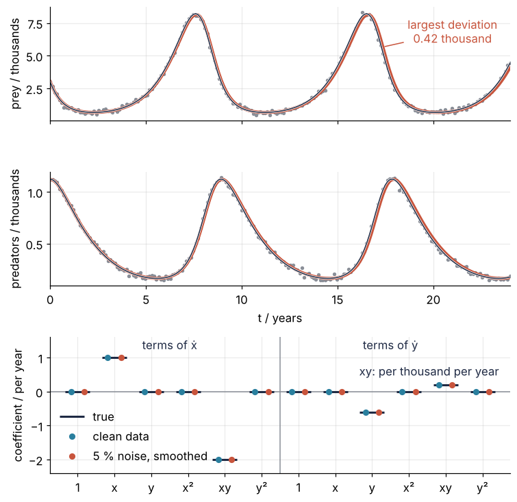
Prey and predators in thousands over 24 years: data with 5 % noise as gray dots, the clean trajectory a thin dark line, the PySINDy model red, lagging slightly after year 16, largest prey deviation 0.42 thousand. Below: the twelve coefficients, true values as bars, clean and noisy fits as dots.

The red curves fall a little behind the dark ones on the way down from the second prey peak, by 0.42 thousand prey near year 17. The red dots sit on the bars.

Pitfalls

A threshold larger than a true coefficient, through your units. Count the prey in hundreds, and \(\delta\) becomes 0.02 per hundred per year, below the default threshold:

X_h = X * [10, 1]                                             # prey in hundreds
with warnings.catch_warnings(record=True) as caught:
    warnings.simplefilter("always")
    ps.SINDy().fit(X_h, t=t, feature_names=["x", "y"]).print()
print("warning:", caught[0].message if caught else "none")

(x)' =  0.219 1 +  0.990 x + -0.446 y + -1.981 x y
(y)' =  0.000
warning: Sparsity parameter is too big (0.1) and eliminated all coefficients

The predator equation is gone and the prey equation has two spurious terms. The threshold is absolute, in the units of the coefficients, and the cliff of Step 3 does the rest. Divide each variable by its mean before fitting, X_h / X_h.mean(axis=0), which returns 0.996 x - 0.982 xy and -0.598 y + 0.523 xy. To convert back, multiply a coefficient by the scale of its equation's variable and divide by the scales of the variables in its term. With the means \(s_x = 26.2\) hundred and \(s_y = 0.493\) thousand, \(\delta = 0.523\,s_y/(s_x s_y) = 0.523/26.2 = 0.0199\) per hundred per year and \(\beta = 0.982\,s_x/(s_x s_y) = 0.982/0.493 = 1.99\). The rates \(\alpha\) and \(\gamma\), whose term is the equation's own variable, stay as they are.

One orbit and a rich library. Allow terms up to degree three, ten per equation, on the same single trajectory:

model_3 = ps.SINDy(feature_library=ps.PolynomialLibrary(degree=3))
model_3.fit(X, t=t, feature_names=["x", "y"])
model_3.print()
print(f"score R² = {model_3.score(X, t=t):.3f}")
print(deviation(model_3.simulate(X[0], t), X))

(x)' =  0.996 x + -1.993 x y
(y)' = -0.761 y^2 +  0.256 x y^2
score R² = 0.950
largest deviation: prey 7.160, predators 0.907 thousand

A score of 0.950, a wrong predator equation, and a simulation off by 7.2 thousand prey. The orbit closes because \(V = \delta x - \gamma \ln x + \beta y - \alpha \ln y\) stays constant along it, so all 200 samples lie on one curve of constant \(V\). A cubic in \(x\) and \(y\) can trace that curve closely: scale each of the ten terms to an rms of 1 over the samples, and one combination of them, with coefficients of unit length, has an rms of only 0.0003. Add any multiple of it to an equation and the rates hardly change, so the regression cannot tell its terms apart. For the six terms of degree two the smallest such combination is 0.033, a hundred times larger. Record from several starting points and pass the trajectories as lists, fit([X1, X2, X3, X4], t=[t1, t2, t3, t4]); PySINDy 2.x has no multiple_trajectories flag. Four trajectories of 50 samples from the phase portrait's starting points give the four true terms within 0.0022. A score near 1 is not a check; a simulation is.

A smoothing window as wide as the peaks. The prey stay above half their peak height for 2.6 years per cycle. The default window of 11 samples spans 1.2 years, under half of that; a window of 21 samples spans 2.4 years, nearly the whole peak. A cubic over such a window cannot bend fast enough to follow the peak and flattens it, even without noise:

wide = ps.SmoothedFiniteDifference(smoother_kws={"window_length": 21})
ps.SINDy(differentiation_method=wide).fit(X, t=t, feature_names=["x", "y"]).print()
print(f"prey peak: data {X[:, 0].max():.2f}, smoothed {wide.smoothed_x_[:, 0].max():.2f} thousand")

(x)' =  0.189 1 +  0.905 x + -0.295 y + -1.787 x y + -0.163 y^2
(y)' = -0.589 y +  0.194 x y
prey peak: data 8.22, smoothed 8.00 thousand

Three spurious terms on clean data, and at 2 % noise none of 20 realizations finds the true model. Plot the smoothed data, smoothed_x_ after a call, over the raw data, and shrink the window until the peaks survive.

Variations

A control input. fit(X, t=t, u=U) and simulate(x0, t, u=U) identify a system driven from outside, for instance prey harvested at a rate \(u(t)\) you set. The library then contains terms in the input too, which is SINDy with control.
Terms that are not polynomials. ps.CustomLibrary(library_functions=[lambda x: x / (1 + x)], function_names=[lambda x: f"{x}/(1+{x})"]) adds the saturating response of Step 2. Combine it with the polynomials by ps.PolynomialLibrary(degree=2) + custom.
The weak form for heavier noise. ps.WeakPDELibrary(function_library=ps.PolynomialLibrary(degree=2), spatiotemporal_grid=t) integrates the equations against smooth test functions instead of differentiating the data, the way past Step 6's limit.
Which terms are certain. ps.EnsembleOptimizer(ps.STLSQ(threshold=0.1), bagging=True, n_models=50) fits 50 models on resampled data. model.optimizer.coef_list holds their coefficients, and the fraction of models in which a term is nonzero is its inclusion frequency.

Cheat sheet

model = ps.SINDy(
    feature_library=ps.PolynomialLibrary(degree=2),       # the terms your mechanism allows
    optimizer=ps.STLSQ(threshold=0.1),                    # below the smallest coefficient, in your units
    differentiation_method=ps.SmoothedFiniteDifference()) # FiniteDifference(order=4) for clean data
model.fit(X, t=t, feature_names=["x", "y"])               # X: rows are times; lists for several runs
model.print(precision=3)
model.get_feature_names(), model.coefficients()           # one row of coefficients per equation
X_sim = model.simulate(X[0], t)                           # the real check, not model.score