Von Neumann stability analysis with SymPy: the leapfrog Courant limit

The problem: why does leapfrog need C ≤ 1?

The wave equation with leapfrog finite differences sent a pulse along a string and watched it blow up at the Courant number C = cΔt/Δx = 1.01. The error grew by a factor of 1.32 per step, against a predicted 1.327, and the tutorial quoted both that factor and the limit C ≤ 1 without deriving them. The scheme is

\[u_j^{n+1} = 2u_j^n - u_j^{n-1} + C^2\left(u_{j+1}^n - 2u_j^n + u_{j-1}^n\right),\]

and nothing in it says why the limit is 1, or why it holds for every wavelength the grid can carry.

Von Neumann stability analysis answers both, and SymPy does the algebra. A linear scheme with constant coefficients on a periodic or unbounded grid maps each Fourier mode \(e^{ikj\Delta x}\) onto itself, multiplied by a factor \(G\) per step. The scheme is stable when no mode has \(|G| > 1\). For leapfrog, \(G\) is a root of

\[G^2 - 2\left(1 - 2C^2\sin^2\frac{k\Delta x}{2}\right)G + 1 = 0,\]

and the shortest wave on the grid, two points per wavelength, sets the limit C ≤ 1. At C = 1.1 that wave grows by a factor of 2.43 per step. The same steps give r = DΔt/Δx² ≤ 1/2 for the explicit heat scheme, show Crank-Nicolson stable for every r, and expand the phase of \(G\) into the lag of short waves.

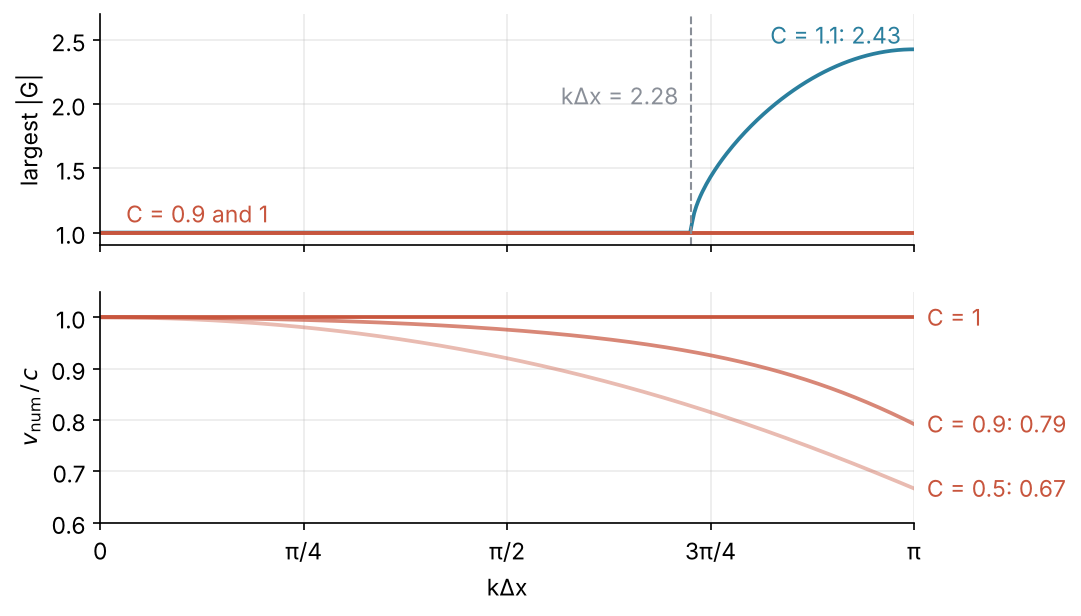
Two panels over kΔx from 0 to π. Top: largest amplification factor |G|; C = 0.9 and 1 stay at 1, C = 1.1 leaves 1 at kΔx = 2.28 and reaches 2.43 at π. Bottom: numerical over true phase speed; C = 1 stays at 1, C = 0.9 and 0.5 lag more as the waves get shorter.

The top panel is the stability limit, the bottom one the numerical dispersion below it. Step 6 draws both from the expressions SymPy derives in Steps 3 and 6.

Setup

The symbols carry assumptions, as in SymPy from the ground up: wavenumber, spacings, and parameters are positive, the grid indices are integers, and \(G\) has none, because it is complex. From Step 3 on, s stands for sin(kΔx/2) and theta for kΔx.

import numpy as np
import sympy as sp
import matplotlib.pyplot as plt

plt.rcParams.update({
    "figure.figsize": (7, 4.4), "figure.dpi": 110,
    "axes.spines.top": False, "axes.spines.right": False,
    "axes.grid": True, "grid.alpha": 0.25,
    "font.size": 11, "lines.linewidth": 1.8,
})
INK, ACCENT, SECOND, MUTED = "#1f2a44", "#c8553d", "#2a7f9e", "#8a8f98"

G = sp.symbols("G")
k, dx, dt, c, C, r, D = sp.symbols("k Delta_x Delta_t c C r D", positive=True)
s, theta = sp.symbols("s theta", positive=True)
j, n = sp.symbols("j n", integer=True)
u = sp.Function("u")

print(f"SymPy {sp.__version__}")

SymPy 1.14.0

Step 1: Write the scheme as an expression in grid values

A grid value \(u_j^n\) is a function of two integer indices, so an undefined SymPy function of two arguments stands for it: u(j + 1, n) is the right neighbor at the current time level. Write the scheme as a residual, the discretized wave equation with everything on one side, which the computed solution makes zero:

\[\frac{u_j^{n+1} - 2u_j^n + u_j^{n-1}}{\Delta t^2} - c^2\,\frac{u_{j+1}^n - 2u_j^n + u_{j-1}^n}{\Delta x^2}.\]

leapfrog = ((u(j, n + 1) - 2 * u(j, n) + u(j, n - 1)) / dt**2
            - c**2 * (u(j + 1, n) - 2 * u(j, n) + u(j - 1, n)) / dx**2)
print(leapfrog)

-c**2*(-2*u(j, n) + u(j - 1, n) + u(j + 1, n))/Delta_x**2 + (-2*u(j, n) + u(j, n - 1) + u(j, n + 1))/Delta_t**2

SymPy keeps the stencil as written, only sorted. This is the one line that changes for another scheme, as Step 5 shows.

Step 2: Put in one Fourier mode and divide out the common factor

One mode is enough because the scheme is linear with constant coefficients. Any grid function is a sum of modes \(e^{ikj\Delta x}\), the scheme maps each of them onto itself, and so the trial solution \(u_j^n = G^n e^{ikj\Delta x}\) tells you everything about growth: the factor \(G(k)\) per step.

Two calls are new since the SymPy tutorial. replace takes a function and calls it with the arguments of every u(...) it finds, so one call covers all five grid values, where subs would need one dictionary entry per grid value. powsimp merges powers of the same base, G**(n + 1)/G**n into G; without the call the powers stay apart. Then multiply by Δt² and by G, which clears the 1/G that \(u_j^{n-1}\) leaves, and put in Δt = CΔx/c:

mode = leapfrog.replace(u, lambda jj, nn: G**nn * sp.exp(sp.I * k * jj * dx))
P = sp.powsimp(sp.expand(mode / (G**n * sp.exp(sp.I * k * j * dx))))
P = sp.expand(sp.expand(P * dt**2 * G).subs(dt, C * dx / c))
print(P)

-C**2*G*exp(I*Delta_x*k) + 2*C**2*G - C**2*G*exp(-I*Delta_x*k) + G**2 - 2*G + 1

The indices j and n are gone, and c, Δt, and Δx survive only inside C and the product kΔx. That is why C is the only knob: two grids with the same Courant number have the same stability.

Step 3: Turn the exponentials into a cosine and solve for G

The two exponentials \(e^{\pm ik\Delta x}\) add up to a cosine. rewrite(sp.cos) writes each in cosines and sines, trigsimp cancels the sines, and collect sorts by powers of \(G\). Step 4 needs an inequality in a plain symbol, so the half-angle identity cos(kΔx) = 1 − 2 sin²(kΔx/2) then puts in s:

P_cos = sp.collect(sp.trigsimp(P.rewrite(sp.cos)), G)
print(P_cos)
P = sp.collect(sp.expand(P_cos.subs(sp.cos(k * dx), 1 - 2 * s**2)), G)
print(P)

G1, G2 = sp.solve(P, G)
print("G1 =", G1)
print("G2 =", G2)
print("G1 * G2 =", sp.simplify(G1 * G2))

G**2 + G*(-2*C**2*cos(Delta_x*k) + 2*C**2 - 2) + 1
G**2 + G*(4*C**2*s**2 - 2) + 1
G1 = -2*C**2*s**2 - 2*C*s*sqrt(C**2*s**2 - 1) + 1
G2 = -2*C**2*s**2 + 2*C*s*sqrt(C**2*s**2 - 1) + 1
G1 * G2 = 1

That is the polynomial from the problem. The product of the roots of a monic quadratic is its constant term (Vieta), here 1, so \(|G_1|\,|G_2| = 1\). Either both roots lie on the unit circle, or one lies outside it and that mode grows.

Step 4: Find the Courant limit at the worst wavenumber

A quadratic with real coefficients and a negative discriminant has a complex conjugate pair of roots, of equal modulus, and with product 1 that modulus is 1. A positive discriminant gives two real roots, and product 1 puts one of them outside the unit circle. So the condition is a discriminant of at most zero, and reduce_inequalities solves it for C:

disc = sp.factor(sp.discriminant(P, G))
print("discriminant:", disc)
print("stable for:  ", sp.reduce_inequalities(disc <= 0, C))

discriminant: 16*C**2*s**2*(C*s - 1)*(C*s + 1)
stable for:   C <= 1/s

The bound depends on the mode. s = sin(kΔx/2) is at most 1, reached at kΔx = π, the shortest wave the grid can carry, so every mode is stable only for C ≤ 1. At C = 1 and kΔx = π the discriminant is zero and the two roots coincide; whether the closed bound is safe is Pitfall 3, and for the clamped string of the leapfrog tutorial it is. Past the limit:

for C_val in [sp.Rational(101, 100), sp.Rational(11, 10)]:
    roots = [sp.N(g.subs({C: C_val, s: 1}), 4) for g in (G1, G2)]
    print(f"C = {float(C_val):.2f}   G at kΔx = π: {roots[0]}, {roots[1]}")
print(f"C = 1.1 unstable from kΔx = {sp.N(2 * sp.asin(1 / sp.Rational(11, 10)), 4)}")

C = 1.01   G at kΔx = π: -1.327, -0.7538
C = 1.10   G at kΔx = π: -2.428, -0.4118
C = 1.1 unstable from kΔx = 2.282

At C = 1.01 one root is −1.327, the factor the leapfrog tutorial predicted and measured as 1.32. The minus sign means the mode flips sign at every step, the alternation that tutorial saw in the error. At C = 1.1 the factor is −2.428, and every wave with kΔx above 2 arcsin(1/1.1) = 2.282, below 2π/2.282 = 2.753 points per wavelength, grows.

Step 5: Run the same steps on the heat equation and Crank-Nicolson

The heat equation \(\partial_t u = D\,\partial_x^2 u\) has two standard schemes. With \(\delta^2 u_j = u_{j+1} - 2u_j + u_{j-1}\), the explicit one steps forward in time with the old second difference,

\[\frac{u_j^{n+1} - u_j^n}{\Delta t} = D\,\frac{\delta^2 u_j^n}{\Delta x^2},\]

and Crank-Nicolson averages the second difference over the old and the new level, which makes each step a linear solve (Finite differences and Crank-Nicolson for the Schrödinger equation build both):

\[\frac{u_j^{n+1} - u_j^n}{\Delta t} = D\,\frac{\delta^2 u_j^n + \delta^2 u_j^{n+1}}{2\Delta x^2}.\]

Steps 2 and 3 go into one function. It takes the residual and the value to put in for Δt, CΔx/c for the wave or rΔx²/D for heat, so that r = DΔt/Δx² is the only parameter left, as C was. It clears the denominators and returns the polynomial in \(G\) divided by its leading coefficient; solve is up to the caller. Leapfrog goes first, as the check:

def amplification(scheme, dt_value):
    mode = scheme.replace(u, lambda jj, nn: G**nn * sp.exp(sp.I * k * jj * dx))
    expr = sp.powsimp(sp.expand(mode / (G**n * sp.exp(sp.I * k * j * dx))))
    expr = sp.trigsimp(sp.expand(expr).rewrite(sp.cos)).subs(dt, dt_value)
    expr = sp.numer(sp.together(expr.subs(sp.cos(k * dx), 1 - 2 * s**2)))
    return sp.collect(sp.Poly(expr, G).monic().as_expr(), G)

print("leapfrog:", amplification(leapfrog, C * dx / c))

d2 = lambda m: u(j + 1, m) - 2 * u(j, m) + u(j - 1, m)
heat = {
    "explicit": (u(j, n + 1) - u(j, n)) / dt - D * d2(n) / dx**2,
    "Crank-Nicolson": (u(j, n + 1) - u(j, n)) / dt - D * (d2(n) + d2(n + 1)) / (2 * dx**2),
}
for name, scheme in heat.items():
    (g,) = sp.solve(amplification(scheme, r * dx**2 / D), G)
    print(f"{name:15s} G = {g}   stable for: {sp.reduce_inequalities(g**2 <= 1, r)}")

leapfrog: G**2 + G*(4*C**2*s**2 - 2) + 1
explicit        G = -4*r*s**2 + 1   stable for: r <= 1/(2*s**2)
Crank-Nicolson  G = (-2*r*s**2 + 1)/(2*r*s**2 + 1)   stable for: True

Leapfrog gives back Step 3's polynomial. The explicit scheme has one root, 1 − 4rs², and its bound r ≤ 1/(2s²) becomes r ≤ 1/2 at s = 1, the limit Finite differences found from the zigzag. Crank-Nicolson's answer is True: stable for every r and every mode. The inequality is squared because \(G\) is real here and the square says the same; on the absolute value of the Crank-Nicolson root, reduce_inequalities raises NotImplementedError in SymPy 1.14.

Step 6: Expand the phase of G for the numerical dispersion, and draw both

An exact wave \(e^{i(kx - \omega t)}\) is multiplied by \(e^{-i\omega\Delta t}\) per step, so a scheme's frequency is read off its root: \(\varphi = \omega\Delta t = -\arg G\), taken on a physical root, one that goes to 1 as kΔx → 0. Leapfrog has two such roots, a right-moving wave with Im G < 0 and its mirror image. The ratio of numerical to true phase speed is \(v_\text{num}/c = \varphi/(C\,k\Delta x)\), and series in kΔx gives the lag of short waves. The phase rule holds for any scheme, the speed ratio for wave and advection schemes, where C exists.

Near kΔx = 0, Re G > 0 and φ = atan(−Im G/Re G). SymPy cannot split leapfrog's root, not knowing the sign under its square root. For Cs ≤ 1 the roots are a conjugate pair with product 1, so Re G is half their sum 2 − 4C²s², and |G| = 1 gives Im G = −√(1 − (Re G)²) = −2Cs√(1 − C²s²):

re_G = 1 - 2 * C**2 * s**2
im_G = -2 * C * s * sp.sqrt(1 - C**2 * s**2)
ratio = (sp.atan(-im_G / re_G) / (C * theta)).subs(s, sp.sin(theta / 2))

series = sp.series(ratio, theta, 0, 5)
print(series)
print("θ² coefficient:", sp.factor(series.removeO().coeff(theta, 2)))
print("θ⁴ coefficient:", sp.factor(series.removeO().coeff(theta, 4)))

at = {C: sp.Rational(1, 2), theta: sp.pi / 3}
closed = 2 * sp.asin(C * sp.sin(theta / 2)) / (C * theta)
print(f"C = 0.5, six points per wavelength: exact {sp.N(ratio.subs(at), 4)}, "
      f"series {sp.N(series.removeO().subs(at), 4)}, closed form {sp.N(closed.subs(at), 4)}")

1 + theta**2*(C**2/24 - 1/24) + theta**4*(3*C**4/640 - C**2/192 + 1/1920) + O(theta**5)
θ² coefficient: (C - 1)*(C + 1)/24
θ⁴ coefficient: (C - 1)*(C + 1)*(3*C - 1)*(3*C + 1)/1920
C = 0.5, six points per wavelength: exact 0.9652, series 0.9651, closed form 0.9652

Both coefficients vanish at C = 1, where leapfrog is exact on the grid; below 1 short waves lag by (1 − C²)(kΔx)²/24. At six points per wavelength and C = 0.5 the series gives 0.9651 against the exact 0.9652, and the closed form φ = 2 arcsin(C sin(kΔx/2)) the leapfrog tutorial quoted gives its 3.5 % lag.

For the figure, lambdify evaluates the roots on complex input (|G| = 1 puts a negative number under the root) and the phase with atan2, since atan jumps by π where Re G turns negative:

roots_np = sp.lambdify((theta, C), [g.subs(s, sp.sin(theta / 2)) for g in (G1, G2)], "numpy")
phi_np = sp.lambdify((theta, C), sp.atan2(-im_G, re_G).subs(s, sp.sin(theta / 2)), "numpy")

th = np.linspace(np.pi / 400, np.pi, 400)
alpha = {0.5: 0.4, 0.9: 0.7, 1.0: 1.0}
fig, (ax_g, ax_v) = plt.subplots(2, 1, sharex=True, figsize=(7, 4.4))

for C_val in [1.1, 0.9, 1.0]:                # the stable curves drawn on top
    G_max = np.max(np.abs(roots_np(th + 0j, C_val)), axis=0)
    color = SECOND if C_val > 1 else ACCENT
    ax_g.plot(th, G_max, color=color, alpha=alpha.get(C_val, 1.0))
onset = 2 * np.arcsin(1 / 1.1)
ax_g.axvline(onset, color=MUTED, ls="--", lw=1)
ax_g.text(onset - 0.05, 2.0, f"kΔx = {onset:.2f}", color=MUTED, ha="right")
ax_g.text(np.pi - 0.05, 2.43, "C = 1.1: 2.43", color=SECOND, ha="right", va="bottom")
ax_g.text(0.1, 1.08, "C = 0.9 and 1", color=ACCENT)
ax_g.set(ylabel="largest |G|", ylim=(0.9, 2.7))

for C_val in [0.5, 0.9, 1.0]:
    v_ratio = phi_np(th, C_val) / (C_val * th)
    ax_v.plot(th, v_ratio, color=ACCENT, alpha=alpha[C_val])
    label = f"C = {C_val:g}" + (f": {v_ratio[-1]:.2f}" if C_val < 1 else "")    # the lag at kΔx = π
    ax_v.text(np.pi + 0.05, v_ratio[-1], label, color=ACCENT, va="center")
ax_v.set(xlabel="kΔx", ylabel=r"$v_\mathrm{num}\,/\,c$", ylim=(0.6, 1.05), xlim=(0, np.pi),
         xticks=np.linspace(0, np.pi, 5), xticklabels=["0", "π/4", "π/2", "3π/4", "π"])
plt.show()

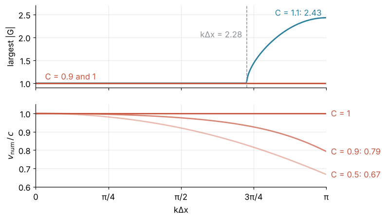
Two panels over kΔx from 0 to π. Top: largest amplification factor |G|; C = 0.9 and 1 stay at 1, C = 1.1 leaves 1 at kΔx = 2.28 and reaches 2.43 at π. Bottom: numerical over true phase speed; C = 1 stays at 1, C = 0.9 and 0.5 lag more as the waves get shorter.

C = 0.9 and 1 stay on |G| = 1, C = 1 only just: at kΔx = π its roots meet in the double root of Pitfall 3. Below, C = 0.5 carries the shortest wave at two thirds of the true speed, C = 0.9 at 0.79.

Pitfalls

Symbols without assumptions. The modulus of \(e^{ik\Delta x}\) is 1, but not for plain symbols:

k_plain, dx_plain = sp.symbols("k Delta_x")
print(sp.Abs(sp.exp(sp.I * k_plain * dx_plain)), "  vs  ", sp.Abs(sp.exp(sp.I * k * dx)))

exp(-im(Delta_x*k))   vs   1

SymPy must allow complex k and Δx, so the modulus stays exp(−Im(kΔx)), and every modulus built on it stays unsimplified. Declare such symbols real or positive, as in the setup.

Checking one wavenumber. You test kΔx = π/2, the obvious medium wave, and solve the discriminant at s = sin(π/4):

print(sp.reduce_inequalities(disc.subs(s, sp.sin(sp.pi / 4)) <= 0, C))

C <= sqrt(2)

A time step 41 % too large passes the check. Keep s symbolic as in Step 4 and take the smallest bound over 0 < s ≤ 1. Written in sin(kΔx/2) instead of s, Step 4's inequality raises NotImplementedError in SymPy 1.14, which is the other reason s is a symbol.

Reading |G| = 1 as stable when the root is double. At C = 1 and kΔx = π, solve returns one root, −1, of modulus 1. roots returns it with its multiplicity:

P_edge = P.subs({C: 1, s: 1})
print(sp.solve(P_edge, G), sp.roots(P_edge, G))

a = [0, 1]                        # the recurrence with characteristic polynomial P_edge
for _ in range(199):
    a.append(-2 * a[-1] - a[-2])
print(f"|a_200| = {abs(a[200])}")

[-1] {-1: 2}
|a_200| = 200

A two-level recurrence with a double root −1 has the solution n(−1)ⁿ, which grows linearly, as an ODE with a repeated characteristic root λ has \(t e^{\lambda t}\). Here it reaches 200 after 200 steps. The leapfrog tutorial is safe at C = 1 because its string has clamped ends: its modes are sin(mπj/N) with m < N, and kΔx = π never occurs. On a periodic grid with an even number of points it does. Whenever a bound is reached with equality, check the multiplicity with roots.

Variations

Upwind advection. The scheme \(u_j^{n+1} = u_j^n - C(u_j^n - u_{j-1}^n)\) of Finite volumes has a single root \(G = 1 - C(1 - e^{-ik\Delta x})\), which as_real_imag() splits, and the limit is 0 ≤ C ≤ 1. Step 6's rule gives \(v_\text{num}/c\) = 1 − (1 − C)(1 − 2C)(kΔx)²/6, exact phase at C = 1/2 and 1, while |G| < 1 damps the short waves.
A fourth-order stencil in space. Replace δ² by \((-u_{j+2} + 16u_{j+1} - 30u_j + 16u_{j-1} - u_{j-2})/12\). The worst mode is still kΔx = π, and the limit drops to C ≤ √3/2 ≈ 0.866.
The Schrödinger equation with Crank-Nicolson. The scheme of Crank-Nicolson for the Schrödinger equation has a \(G\) that is a ratio of complex conjugates, so |G| = 1 exactly for every step size.
A membrane. Two wavenumbers, \(u(j, l, n)\), and the five-point Laplacian. The worst mode is (π, π), and the limit is C ≤ 1/√2, the value the leapfrog tutorial quotes.

Cheat sheet

u = sp.Function("u")                                   # u(j, n): grid value; k, dx positive; scheme = residual
mode = scheme.replace(u, lambda j_, n_: G**n_ * sp.exp(sp.I * k * j_ * dx))
P = sp.powsimp(sp.expand(mode / (G**n * sp.exp(sp.I * k * j * dx))))
P = sp.trigsimp(P.rewrite(sp.cos)).subs(sp.cos(k * dx), 1 - 2 * s**2)   # s = sin(kΔx/2)
sp.solve(P, G); sp.roots(P, G)                         # roots; roots() shows multiplicity
sp.factor(sp.discriminant(P, G))       # monic quadratic with constant term 1: stable where <= 0
sp.reduce_inequalities(g**2 <= 1, r)                   # one real root; then worst mode s = 1
re_G, im_G = g.as_real_imag()          # one root; pair with product 1: re_G = sum/2, im_G = -sqrt(1 - re_G**2)
phi = sp.atan(-im_G / re_G)            # on the root with G -> 1 as kΔx -> 0; valid while re_G > 0
sp.series((phi / (C * theta)).subs(s, sp.sin(theta / 2)), theta, 0, 5)   # v_num / c