Monte Carlo transport: why a shield lets through more than e⁻³ (Python)

The question

A beam of neutrons falls on a shield three mean free paths thick. The mean free path is the average distance a neutron flies between two collisions, and the exponential attenuation law says which fraction of the beam crosses without a single one: e⁻³ = 4.98 %. A detector behind the shield, counting every neutron that leaves the far face at any angle, reads more than that, because a collision does not always remove the neutron. Here are 40 neutrons in a slab where nine collisions in ten scatter the neutron into a new direction and one in ten absorbs it:

Show code

import numpy as np
import matplotlib.pyplot as plt
from scipy.integrate import quad
from scipy.special import expn

plt.rcParams.update({
    "figure.figsize": (7, 3.6), "figure.dpi": 110,
    "axes.spines.top": False, "axes.spines.right": False,
    "axes.grid": True, "grid.alpha": 0.25,
    "font.size": 11, "lines.linewidth": 1.8,
})
INK, ACCENT, SECOND, MUTED = "#1f2a44", "#c8553d", "#2a7f9e", "#8a8f98"

# The neutrons below are simulated by the method this tutorial explains, so that the
# answer can be checked at the end. Pretend you have not seen this cell.
# Lengths are in mean free paths throughout.
rng = np.random.default_rng(2026)


def history(tau, c, rng):
    """One neutron through a slab of thickness tau: fate, collisions, track, exit direction."""
    x, y, mu, dy = 0.0, 0.0, 1.0, 0.0           # depth, transverse position, direction cosines
    points = [(x, y)]
    n = 0
    while True:
        s = rng.exponential(1.0)                 # free path, mean 1 mean free path
        x_new = x + mu * s
        if x_new > tau or x_new < 0:             # left through a face: stop the track there
            face = tau if x_new > tau else 0.0
            points.append((face, y + dy * (face - x) / mu))
            return ("T" if face == tau else "R"), n, np.array(points), (mu, dy)
        x, y = x_new, y + dy * s
        points.append((x, y))
        n += 1
        if rng.random() >= c:                    # absorbed
            return "A", n, np.array(points), None
        mu = rng.uniform(-1, 1)                  # isotropic: the cosine is uniform
        dy = np.sqrt(1 - mu**2) * np.cos(rng.uniform(0, 2 * np.pi))   # only for drawing


def draw_tracks(ax, histories, tau):
    """Slab as a band, beam from the left, each track SECOND to its first collision, ACCENT after."""
    ax.axvspan(0, tau, color=MUTED, alpha=0.12, lw=0)
    ax.plot([-2, 0], [0, 0], color=SECOND, lw=1)
    for fate, n, p, direction in histories:
        ax.plot(p[:2, 0], p[:2, 1], color=SECOND, lw=1, alpha=0.8)
        ax.plot(p[1:, 0], p[1:, 1], color=ACCENT, lw=1, alpha=0.8)
        if fate == "A":
            ax.plot(*p[-1], "x", color=MUTED, ms=6, mew=1.6, zorder=3)
        else:                                    # a short stub outside the face it left through
            end = p[-1] + 0.8 * np.array(direction)
            ax.plot([p[-1, 0], end[0]], [p[-1, 1], end[1]], color=SECOND if n == 0 else ACCENT, lw=1, alpha=0.8)
    ax.set(xlim=(-1.5, tau + 1.5))


TAU = 3.0
shown = [history(TAU, 0.9, rng) for _ in range(40)]
fig, ax = plt.subplots(figsize=(8, 3.5))
draw_tracks(ax, shown, TAU)
ax.set(ylim=(-3.5, 3.5), xlabel="depth / mean free paths", ylabel="transverse / mean free paths")
plt.show()
drawn = [("T", True), ("T", False), ("R", False), ("A", False)]
counts = [sum((fate, n == 0) == key for fate, n, *_ in shown) for key in drawn]
print("the 40 drawn: {} crossed uncollided, {} crossed after scattering, {} reflected, {} absorbed".format(*counts))

fates, orders = {}, {}
for c in [0.5, 0.9]:
    f, n, *_ = zip(*[history(TAU, c, rng) for _ in range(100_000)])
    fates[c], orders[c] = np.array(f), np.array(n)
    crossed = fates[c] == "T"
    print(f"c = {c}:  uncollided {np.mean(crossed & (orders[c] == 0)):6.2%}   "
          f"crossed in total {np.mean(crossed):6.2%}   reflected {np.mean(fates[c] == 'R'):6.2%}")
print(f"exponential law e^-3 = {np.exp(-TAU):.2%}")

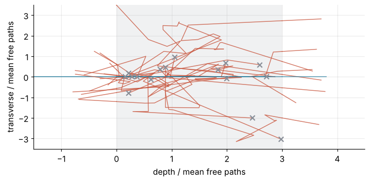
Forty neutron tracks through a slab 3 mean free paths thick, depth against transverse position in mean free paths. The beam enters from the left; one track crosses straight, 8 cross after scattering, and 15 bend back out through the front face.

the 40 drawn: 1 crossed uncollided, 8 crossed after scattering, 15 reflected, 16 absorbed
c = 0.5:  uncollided  4.86%   crossed in total  7.68%   reflected 11.65%
c = 0.9:  uncollided  4.99%   crossed in total 21.35%   reflected 39.70%
exponential law e^-3 = 4.98%

Every track enters from the left along the beam, blue until its first collision and red after it. A gray cross marks an absorption, and a stub outside a face marks where a track left the slab. Of these 40, one crosses straight, eight cross after scattering, and 15 come back out through the front face. The rest of the printout follows 100,000 neutrons through each of two materials, whose collisions scatter half the time and nine times in ten.

Two things are obvious. The straight tracks cross at the rate of the exponential law: 4.86 % cross uncollided in the first material and 4.99 % in the second, against 4.98 %. A fraction counted from 100,000 neutrons varies by about 0.07 % from seed to seed, its standard error, so both agree. The bent tracks cross too, and even more of them turn around: 39.70 % of all neutrons leave through the front face when nine collisions in ten scatter.

Less obvious: in total 7.68 % cross when half the collisions scatter and 21.35 % when nine in ten do. The detector sees one neutron in five where the exponential law promised one in twenty. Why does the scattering ratio make that much difference between 0.5 and 0.9, and why is there no formula as short as e⁻³ for the total? Every shield design has to answer this, because a detector, or a person, behind the shield counts all the neutrons, not only the straight ones.

The idea: follow one neutron, three random draws per flight

Follow one neutron. Its life in the slab is a sequence of flights, and each flight takes three random numbers: how far it goes, what happens when it stops, and where it goes next. Lengths are in mean free paths from here on, so the slab is τ = 3 mean free paths thick.

How far. The chance of flying further than a distance ℓ without a collision is $e^{-\Sigma_t \ell}$, where $\Sigma_t$, the total macroscopic cross section, is the chance of a collision per centimeter of path and $1/\Sigma_t$ is the mean free path. Draw a uniform number U between 0 and 1 and set the free path to $s = -\ln(U)/\Sigma_t$. Then s exceeds ℓ exactly when U is below $e^{-\Sigma_t \ell}$, and a uniform number is below any p with probability p, so the drawn paths survive at exactly the rate of the exponential law. NumPy does it in one call, rng.exponential(scale=1/sigma_t, size=n), and scale is the mean of the distribution, the mean free path, not the rate $\Sigma_t$. Here lengths are in mean free paths, so the scale is 1; on your own problem in centimeters you pass $1/\Sigma_t$. Pass $\Sigma_t$ by mistake and you get a mean flight of $\Sigma_t$ instead of $1/\Sigma_t$, with no error message.

What happens. At the end of the flight the neutron collides. With probability c, the scattering ratio, it scatters and flies on; otherwise it is absorbed and its history ends. rng.random(n) < c makes that decision for n neutrons at once.

Where next. Isotropic scattering means that every direction on the sphere is equally likely. Cut the unit sphere into bands of equal height dμ along the slab's normal: Archimedes showed that each band has the same area, 2π dμ, whether it sits at the equator or near a pole. Equal heights hold equal shares of the directions, so the direction cosine μ, the cosine of the angle to the normal, is uniform on [−1, 1], drawn by rng.uniform(-1, 1, size=n). A uniform angle would crowd the directions near the poles, with too many neutrons flying straight ahead or straight back. Neutron moderation makes the same argument with a figure.

In a slab only the depth matters, changed by μs in a flight of length s; the transverse spread in the figures is for the eye. The model is the simplest one that shows the effect: one speed, isotropic scattering, a beam at normal incidence, a slab of infinite width. Real neutrons lose energy in collisions until they are thermal and scatter mostly forward off light nuclei. Here is the same slab with 25 neutrons at three scattering ratios:

Show code

rng_demo = np.random.default_rng(1)                       # its own stream, so the main one stays as it is
fig, axes = plt.subplots(3, 1, figsize=(8, 6.3), sharex=True)
for ax, c in zip(axes, [0.0, 0.5, 0.9]):
    tracks = [history(TAU, c, rng_demo) for _ in range(25)]
    draw_tracks(ax, tracks, TAU)
    ax.text(0.99, 0.95, f"c = {c:g}", transform=ax.transAxes, ha="right", va="top")
    ax.set(ylim=(-3, 3))
axes[-1].set_xlabel("depth / mean free paths")
fig.supylabel("transverse / mean free paths", fontsize=11)
plt.show()

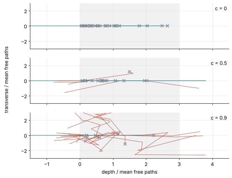
The same slab with 25 neutrons each at scattering ratios c = 0, 0.5, and 0.9. At c = 0 every track is straight and ends at an absorption; at c = 0.9 bent scattered tracks fill the slab and some reach the far face.

With c = 0 the tracks are straight lines that end at their first gray cross, and about one in twenty would reach the far face; of these 25, none does. With c = 0.5 a few neutrons survive a collision and fly off at an angle, and with c = 0.9 the bent tracks fill the front half of the slab and some of them reach the far face. The exponential law is the top panel: it counts every collision as a loss.

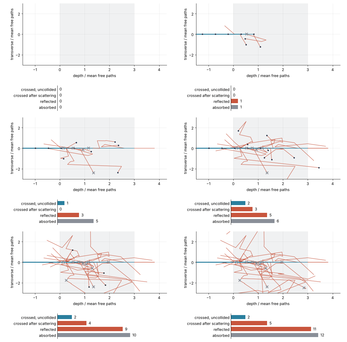
Here are 30 neutrons at c = 0.9, entering one after another and all moving at the same speed, with a tally of how each one ended:

Thirty neutrons enter a 3 mean free path slab one after another with c = 0.9; tracks turn red after their first collision and absorptions leave gray crosses. Bars tally the outcomes: 2 crossed uncollided, 5 crossed after scattering, 11 reflected, 12 absorbed.

Show code

"""Thirty neutrons through a slab three mean free paths thick, nine collisions in ten a scattering.

Top: the tracks as they grow, all neutrons moving at the same speed, so a frame is a moment.
Bottom: the running tally of how each neutron ended.

Renders ../../assets/slab-tracks.gif. Run from this directory:

    python scene.py
"""
from pathlib import Path

import matplotlib
import numpy as np

matplotlib.use("Agg")
import matplotlib.pyplot as plt
from matplotlib.animation import FuncAnimation, PillowWriter

OUT = Path(__file__).resolve().parents[2] / "assets" / "slab-tracks.gif"
INK, ACCENT, SECOND, MUTED = "#1f2a44", "#c8553d", "#2a7f9e", "#8a8f98"

# Same physics as index.md; lengths in mean free paths.
TAU, C, N_NEUTRONS = 3.0, 0.9, 30
START, STUB = -1.5, 0.8                    # where the beam starts, how far a track runs past a face
N_FRAMES, HOLD = 110, 14                   # the last HOLD frames show the finished picture
rng = np.random.default_rng(8)


def history():
    """Points of one track in (depth, transverse), the 3D length of each leg, and the outcome."""
    x, y, mu, dy = 0.0, 0.0, 1.0, 0.0
    points, legs, n = [(START, 0.0), (0.0, 0.0)], [-START], 0
    while True:
        s = rng.exponential(1.0)
        if not 0 <= x + mu * s <= TAU:                     # leaves through a face
            face = TAU if x + mu * s > TAU else 0.0
            s = (face - x) / mu
            points += [(face, y + dy * s), (face + STUB * mu, y + dy * (s + STUB))]
            legs += [s, STUB]
            outcome = "reflected" if face == 0 else ("crossed, uncollided" if n == 0 else "crossed after scattering")
            return np.array(points), np.array(legs), n, outcome
        x, y = x + mu * s, y + dy * s
        points.append((x, y))
        legs.append(s)
        n += 1
        if rng.random() >= C:
            return np.array(points), np.array(legs), n, "absorbed"
        mu = rng.uniform(-1, 1)                            # isotropic: the cosine is uniform
        dy = np.sqrt(1 - mu**2) * np.cos(rng.uniform(0, 2 * np.pi))


tracks = [history() for _ in range(N_NEUTRONS)]
delay = np.arange(N_NEUTRONS) * 2                          # one neutron enters every second frame
# the length up to the event that decides the outcome (face crossing or absorption)
decided = np.array([legs.sum() - (STUB if out != "absorbed" else 0) for _, legs, _, out in tracks])
total = np.array([legs.sum() for _, legs, _, _ in tracks])
speed = max(total / (N_FRAMES - HOLD - delay))              # mean free paths per frame; the slowest ends in time

CATEGORIES = ["crossed, uncollided", "crossed after scattering", "reflected", "absorbed"]
BAR_COLOR = [SECOND, ACCENT, ACCENT, MUTED]          # the colors of the tracks: uncollided, scattered, absorbed

plt.rcParams.update({"font.size": 11, "axes.spines.top": False, "axes.spines.right": False,
                     "axes.grid": True, "grid.alpha": 0.25})
fig = plt.figure(figsize=(7, 4.6), dpi=80)                 # 560 x 368 px
ax = fig.add_axes([0.13, 0.43, 0.83, 0.54])                # tracks
ax_bar = fig.add_axes([0.33, 0.03, 0.63, 0.22])            # tally, room on the left for its labels

ax.axvspan(0, TAU, color=MUTED, alpha=0.12, lw=0)
ax.set(xlim=(START, TAU + 1.3), ylim=(-3, 3), yticks=[-2, 0, 2],
       xlabel="depth / mean free paths", ylabel="transverse / mean free paths")

lines = []
for points, legs, n, outcome in tracks:
    (before,) = ax.plot([], [], color=SECOND, lw=1.2)       # beam and first free path
    (after,) = ax.plot([], [], color=ACCENT, lw=1.2, alpha=0.85)
    (head,) = ax.plot([], [], "o", color=INK, ms=3)
    (cross,) = ax.plot([], [], "x", color=MUTED, ms=7, mew=2, zorder=3)
    lines.append((before, after, head, cross))

bars = ax_bar.barh(range(4), [0] * 4, color=BAR_COLOR, height=0.7)
ax_bar.set(xlim=(0, N_NEUTRONS * 0.5), ylim=(3.6, -0.6), yticks=range(4), yticklabels=CATEGORIES, xticks=[])
ax_bar.grid(False)
ax_bar.spines["bottom"].set_visible(False)                  # the counts are written at the bars
ax_bar.tick_params(axis="y", length=0)
counts_text = [ax_bar.text(0, i, "", va="center", ha="left") for i in range(4)]


def walk(points, legs, d):
    """The track up to distance d along it, as a polyline."""
    edges = np.concatenate([[0], np.cumsum(legs)])
    j = np.searchsorted(edges, d, side="right")             # legs fully done: j - 1
    if j > len(legs):
        return points
    frac = (d - edges[j - 1]) / legs[j - 1]
    tip = points[j - 1] + frac * (points[j] - points[j - 1])
    return np.vstack([points[:j], tip])


def update(frame):
    counts = dict.fromkeys(CATEGORIES, 0)
    for (points, legs, n, outcome), (before, after, head, cross), t0, t_dec in zip(tracks, lines, delay, decided):
        d = (frame - t0) * speed
        if d <= 0:
            continue
        path = walk(points, legs, d)
        before.set_data(path[:3, 0], path[:3, 1])
        after.set_data(path[2:, 0], path[2:, 1])
        done = d >= legs.sum()
        head.set_data([] if done else [path[-1, 0]], [] if done else [path[-1, 1]])
        if d >= t_dec:
            counts[outcome] += 1
            if outcome == "absorbed":
                cross.set_data([points[-1, 0]], [points[-1, 1]])
                head.set_data([], [])
    for i, name in enumerate(CATEGORIES):
        bars[i].set_width(counts[name])
        counts_text[i].set_position((counts[name] + 0.3, i))
        counts_text[i].set_text(str(counts[name]))
    return ()


anim = FuncAnimation(fig, update, frames=range(N_FRAMES), blit=False)
anim.save(OUT, writer=PillowWriter(fps=12))
final = {name: sum(out == name for *_, out in tracks) for name in CATEGORIES}
print("wrote", OUT, OUT.stat().st_size // 1024, "kB; speed", round(speed, 3), "mean free paths per frame;", final)

Of the 30, two cross uncollided and five cross after scattering, 11 leave through the front face, and 12 are absorbed. Scattering is not removal. A neutron knocked out of the beam is still in the slab, and it gets another chance at the far face.

Why the scattered neutrons get through

Sort the neutrons that crossed in the 100,000 histories of the first cell by the number of collisions they had on the way:

Show code

k = np.arange(16)
ACCENT_FAINT = "#de998b"                                  # ACCENT mixed 60:40 with white: less scattering
fig, ax = plt.subplots(figsize=(7, 3.6))
ax.axhline(np.exp(-TAU), color=MUTED, lw=1, ls="--")
ax.text(15, np.exp(-TAU) * 1.15, "e⁻³", color=MUTED, ha="right", va="bottom")
for c, color in [(0.5, ACCENT_FAINT), (0.9, ACCENT)]:
    T_k = np.array([np.mean((fates[c] == "T") & (orders[c] == j)) for j in k])
    keep = (k > 0) & (T_k >= 1e-4)                         # orders with at least 10 neutrons
    ax.plot(k[keep], T_k[keep], "o-", color=color, ms=4, lw=1.2)
    j = 5 if c == 0.5 else 15                             # where the label goes, inside the axes
    ax.text(j + 0.4, T_k[j], f"c = {c}", color=color, va="center")
    print(f"c = {c}:  " + " ".join(f"{t:.4f}" for t in T_k[:11]))
ax.plot(0, np.exp(-TAU), "o", color=SECOND, ms=6)
ax.set(yscale="log", ylim=(1e-4, 0.1), xlabel="collisions before crossing", ylabel="transmitted fraction")
plt.show()

c = 0.5:  0.0486 0.0142 0.0073 0.0036 0.0017 0.0008 0.0003 0.0002 0.0001 0.0000 0.0000
c = 0.9:  0.0499 0.0252 0.0239 0.0210 0.0182 0.0154 0.0131 0.0099 0.0079 0.0063 0.0052

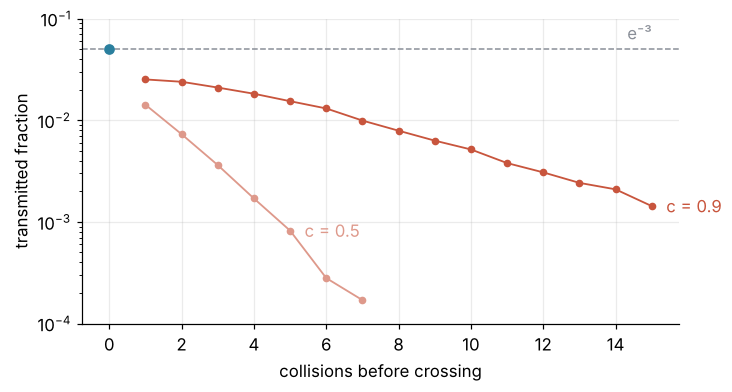
Fraction of neutrons crossing a 3 mean free path slab against the number of collisions on the way, log scale. Zero collisions sits on the dashed e⁻³ line. At c = 0.9 the next orders each bring about half of that and fall slowly; at c = 0.5 each order halves.

Zero collisions is the uncollided beam, one point for both because it does not depend on c. With c = 0.9 the first three scattered orders bring 2.52 %, 2.39 %, and 2.10 %, each about half of the uncollided beam, and the orders fall off slowly after that: neutrons with ten collisions still make up 0.52 %. With c = 0.5 each order brings about half of the one before, 1.42 %, 0.73 %, 0.36 %. Every further collision costs a factor c for surviving it. In return the neutron gets a fresh flight in a fresh direction from somewhere inside the slab, and from there its chance of reaching the far face is far better than e⁻³. Summed, the scattered neutrons are 77 % of what crosses at c = 0.9, and the total is 4.3 times e⁻³. At c = 0.5 it is 1.5 times.

A thicker slab widens the gap. For the beam every collision is a loss, so it falls by a factor e per mean free path. For the neutrons as a whole only a fraction 1 − c of the collisions is a loss, and a neutron that scattered backward may turn forward again in its next collision. So each extra mean free path of slab costs the whole population less than a factor e, and the ratio of all crossing neutrons to the uncollided ones grows with thickness. That ratio is the buildup factor, and the last figure, in the code section below, shows it from 0.5 to 5 mean free paths.

Formalization

The total cross section $\Sigma_t$ is the probability of a collision per unit length, and its inverse $\lambda = 1/\Sigma_t$ is the mean free path. A slab of thickness d is $\tau = \Sigma_t d$ mean free paths thick, its optical thickness. The scattering ratio is $c = \Sigma_s/\Sigma_t$, with $\Sigma_s$ the scattering part of $\Sigma_t$. Free paths have the density on the left, and the expression on the right draws from it with U uniform between 0 and 1:

\[p(s) = \Sigma_t\, e^{-\Sigma_t s}, \qquad s = -\frac{\ln U}{\Sigma_t}.\]

Writing ln(1 − U) instead changes nothing, since U and 1 − U have the same distribution. The direction cosine μ after a collision is uniform on [−1, 1].

The loop samples the solution of the one-speed transport equation, a balance of the neutrons at each depth and in each direction, in which collisions remove neutrons and scattering puts them back in new directions. The putting back is the term the exponential law drops. What crosses splits by the number of collisions, and the buildup factor B is the ratio of all to uncollided:

\[T = T_0 + T_1 + T_2 + \dots, \qquad B = \frac{T}{T_0}.\]

The buildup factors in shielding tables, such as the gamma-ray tables of the ANSI/ANS-6.4.3 standard, are defined for exposure or absorbed energy from a point source in an infinite medium, so their numbers are not these. Here B counts neutrons at the far face of a slab.

The uncollided part is exact and blind to c. T₀ = $e^{-\tau}$, 4.98 % at three mean free paths whether c is 0.5 or 0.9. It is the first check any transport code has to pass.

One scattering is still a short integral; the total is not. With depths in mean free paths,

\[T_1 = \frac{c}{2}\int_0^\tau e^{-x} E_2(\tau - x)\, dx, \qquad E_2(y) = \int_0^1 e^{-y/\mu}\, d\mu .\]

Read it factor by factor. $e^{-x}\,dx$ is the chance that the first collision happens between depth x and x + dx: the beam reaches x uncollided, then collides within dx. c is the chance that this collision scatters, and 1/2 the chance that the new direction points forward, μ > 0, half of [−1, 1]. E₂(τ − x) is the chance to cross the remaining τ − x without another collision, averaged over the forward directions, since a slanted flight has (τ − x)/μ to go; SciPy has it as scipy.special.expn(2, y). The integral adds this up over every depth of the first collision:

Show code

N_Q = 100_000
print("c     T0 exact   T0 simulated      T1 analytic   T1 simulated")
for c in [0.5, 0.9]:
    T0 = np.exp(-TAU)
    T1 = c / 2 * quad(lambda x: np.exp(-x) * expn(2, TAU - x), 0, TAU)[0]
    sim = [np.mean((fates[c] == "T") & (orders[c] == j)) for j in (0, 1)]
    err = [np.sqrt(p * (1 - p) / N_Q) for p in sim]
    print(f"{c}   {T0:.4f}     {sim[0]:.4f} ± {err[0]:.4f}   {T1:.4f}        {sim[1]:.4f} ± {err[1]:.4f}")

c     T0 exact   T0 simulated      T1 analytic   T1 simulated
0.5   0.0498     0.0486 ± 0.0007   0.0143        0.0142 ± 0.0004
0.9   0.0498     0.0499 ± 0.0007   0.0258        0.0252 ± 0.0005

T₁ is 1.43 % at c = 0.5 and 2.58 % at c = 0.9. The once-scattered neutrons of the first cell, 1.42 ± 0.04 % and 2.52 ± 0.05 %, agree within 1.2 standard errors. Every further order can be written the same way, with one more collision depth and one more exponential integral per scattering: T₂ is a double integral over the depths of the first two collisions. Nothing forbids writing them all down, but at c = 0.9 the tenth order still carries 0.52 %, so the total is a sum of ten or more ever deeper integrals. The simulation does the whole sum at once.

The error bar is binomial, and thick shields make it expensive. Each neutron crosses or does not, like a coin that lands heads with probability T, whose variance is T(1 − T). For N neutrons the standard error of the crossed fraction is

\[\sigma_T = \sqrt{\frac{T(1-T)}{N}},\]

which is ± 0.0004 on 0.2150 for 10⁶ neutrons at three mean free paths and c = 0.9. Relative to T it is √((1 − T)/(NT)), and it grows as T falls: 0.19 % at τ = 3 and 0.35 % at τ = 5 in the table below. Solve it for N to see what a 1 % error bar costs on a real shield that lets through T = 10⁻⁶:

Show code

T_shield = 1e-6                                        # a real shield
N_needed = (1 - T_shield) / (T_shield * 0.01**2)       # sigma_T / T = 1 %, solved for N
print(f"neutrons for 1 % relative error at T = {T_shield:g}: {N_needed:.1e}")

neutrons for 1 % relative error at T = 1e-06: 1.0e+10

That is 1.0 × 10¹⁰ histories for one number. Production codes therefore bias the game with splitting, implicit capture, and weight windows, tricks that make rare crossings less rare and carry a weight on each particle to correct for it. Monte Carlo failure probability with an error bar works through the same binomial error and the number of samples a target precision needs.

See it in code

The cell below follows all neutrons at once. transmit(tau, c, n, rng) keeps three arrays, the depth, the direction cosine, and the number of collisions of every neutron still inside. Each pass of its loop draws one free path for each of them with rng.exponential, moves them all, and takes out the neutrons past either face, counting those past the far face as crossed. Of the rest it absorbs a fraction 1 − c with rng.random, gives the survivors a new μ with rng.uniform, and goes around again until no neutron is left inside. It runs 10⁶ neutrons for each thickness from 0.5 to 5 mean free paths and both values of c, checks that crossed, reflected, and absorbed add up to N, and prints the table behind the figure:

Show code

def transmit(tau, c, n, rng):
    """Counts of n neutrons that cross a slab (all, uncollided), are reflected, or absorbed."""
    x, mu, k = np.zeros(n), np.ones(n), np.zeros(n, dtype=int)   # only the neutrons still inside
    n_T = n_T0 = n_R = n_A = 0
    while x.size:
        x = x + mu * rng.exponential(1.0, x.size)        # one free path for every neutron inside
        far, near = x > tau, x < 0
        n_T += far.sum()
        n_T0 += (far & (k == 0)).sum()
        n_R += near.sum()
        inside = ~(far | near)
        x, k = x[inside], k[inside] + 1
        scatter = rng.random(x.size) < c
        n_A += (~scatter).sum()
        x, k = x[scatter], k[scatter]
        mu = rng.uniform(-1, 1, x.size)                  # a new direction for the survivors
    assert n_T + n_R + n_A == n, "neutrons lost"
    return n_T, n_T0, n_R, n_A


N = 1_000_000
taus = np.arange(0.5, 5.01, 0.5)
result = {}
print("  c    τ   uncollided  e^-τ    off by   crossed ± σ        σ/T      B")
for c in [0.5, 0.9]:
    rows = []
    for tau in taus:
        n_T, n_T0, n_R, n_A = transmit(tau, c, N, rng)
        T, T0 = n_T / N, n_T0 / N
        sigma = np.sqrt(T * (1 - T) / N)
        off = (T0 - np.exp(-tau)) / np.sqrt(T0 * (1 - T0) / N)     # in standard errors
        rows.append((T0, T, sigma))
        print(f"{c:4.1f} {tau:4.1f}   {T0:.4f}    {np.exp(-tau):.4f}  {off:+4.1f} σ   {T:.4f} ± {sigma:.4f}   {sigma / T:5.2%}  {T / np.exp(-tau):5.2f}")
    result[c] = np.array(rows)

fig, (ax, ax_B) = plt.subplots(2, 1, figsize=(8, 4.4), sharex=True)
tau_fine = np.linspace(0, 5.2, 200)
ax.plot(tau_fine, np.exp(-tau_fine), color=SECOND, lw=1.6)
ax.plot(taus, result[0.9][:, 0], "o", color=SECOND, mfc="none", ms=6)
ax.text(1.0, 0.012, r"$e^{-\tau}$ and simulated uncollided", color=SECOND, ha="left", va="center")
for c, color in [(0.5, ACCENT_FAINT), (0.9, ACCENT)]:
    T, sigma = result[c][:, 1], result[c][:, 2]
    B = T / np.exp(-taus)
    ax.errorbar(taus, T, yerr=sigma, fmt="o-", color=color, ms=5, lw=1, capsize=2)
    ax_B.plot(taus, B, "o-", color=color, ms=5, lw=1)
    ax.text(5.15, T[-1], f"c = {c}", color=color, ha="left", va="center")
    ax_B.annotate(f"{B[5]:.2f}", (3, B[5]), xytext=(-8, 6), textcoords="offset points",
                  ha="right", color=color)
for a in (ax, ax_B):
    a.axvline(TAU, color=MUTED, lw=1, ls="--")
ax.set(yscale="log", ylim=(3e-3, 1.1), ylabel="transmitted fraction")
ax_B.set(xlim=(0, 5.6), ylim=(0, 12.5), xlabel="thickness τ / mean free paths", ylabel="buildup B")
plt.show()

  c    τ   uncollided  e^-τ    off by   crossed ± σ        σ/T      B
 0.5  0.5   0.6067    0.6065  +0.4 σ   0.6747 ± 0.0005   0.07%   1.11
 0.5  1.0   0.3676    0.3679  -0.7 σ   0.4456 ± 0.0005   0.11%   1.21
 0.5  1.5   0.2231    0.2231  +0.0 σ   0.2917 ± 0.0005   0.16%   1.31
 0.5  2.0   0.1354    0.1353  +0.3 σ   0.1895 ± 0.0004   0.21%   1.40
 0.5  2.5   0.0820    0.0821  -0.2 σ   0.1225 ± 0.0003   0.27%   1.49
 0.5  3.0   0.0496    0.0498  -1.1 σ   0.0783 ± 0.0003   0.34%   1.57
 0.5  3.5   0.0303    0.0302  +0.5 σ   0.0503 ± 0.0002   0.43%   1.67
 0.5  4.0   0.0185    0.0183  +1.2 σ   0.0323 ± 0.0002   0.55%   1.76
 0.5  4.5   0.0112    0.0111  +0.8 σ   0.0203 ± 0.0001   0.69%   1.83
 0.5  5.0   0.0066    0.0067  -1.2 σ   0.0129 ± 0.0001   0.88%   1.91
 0.9  0.5   0.6061    0.6065  -0.8 σ   0.7651 ± 0.0004   0.06%   1.26
 0.9  1.0   0.3675    0.3679  -0.7 σ   0.5916 ± 0.0005   0.08%   1.61
 0.9  1.5   0.2237    0.2231  +1.4 σ   0.4595 ± 0.0005   0.11%   2.06
 0.9  2.0   0.1354    0.1353  +0.1 σ   0.3564 ± 0.0005   0.13%   2.63
 0.9  2.5   0.0817    0.0821  -1.3 σ   0.2763 ± 0.0004   0.16%   3.37
 0.9  3.0   0.0501    0.0498  +1.7 σ   0.2150 ± 0.0004   0.19%   4.32
 0.9  3.5   0.0303    0.0302  +0.5 σ   0.1659 ± 0.0004   0.22%   5.49
 0.9  4.0   0.0182    0.0183  -0.9 σ   0.1285 ± 0.0003   0.26%   7.02
 0.9  4.5   0.0111    0.0111  +0.2 σ   0.0993 ± 0.0003   0.30%   8.94
 0.9  5.0   0.0068    0.0067  +0.6 σ   0.0766 ± 0.0003   0.35%  11.36

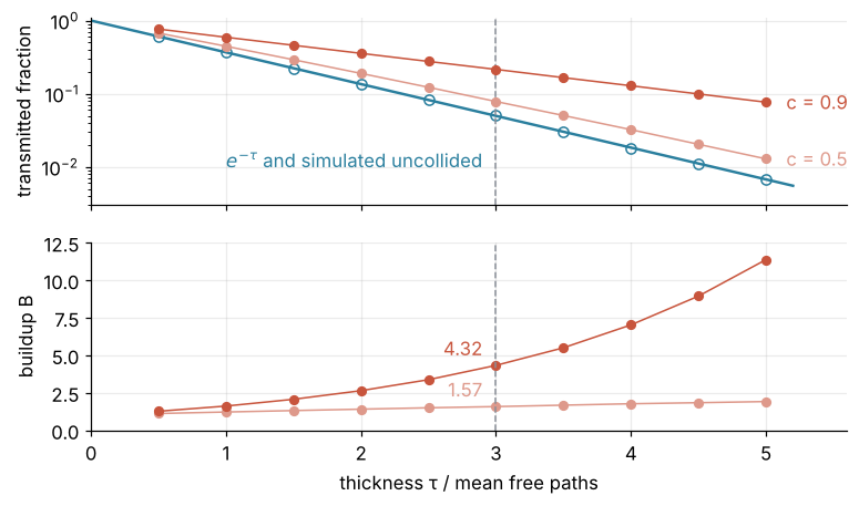
$Top: transmitted fraction against slab thickness, 0.5 to 5 mean free paths, log scale; simulated uncollided points on the exp(−τ) line, totals for c = 0.5 and 0.9 above it. Bottom: buildup factor, 1.57 and 4.32 at 3 mean free paths, reaching 1.91 and 11.36 at 5.$

The uncollided fraction lands on $e^{-\tau}$ at every thickness, 14 of the 20 within one standard error, close to the two in three that honest error bars cover, and all within 1.7. At τ = 3 the totals, 7.83 ± 0.03 % and 21.50 ± 0.04 %, agree with the 7.68 % and 21.35 % of the first cell within two standard errors of that smaller run. The buildup factor grows from 1.11 to 1.91 at c = 0.5 and from 1.26 to 11.36 at c = 0.9, 1.57 and 4.32 at three mean free paths. Each ± shrinks only as 1/√N, which Monte Carlo integration derives.

Where it shows up

Wherever particles or light cross matter that scatters them, the exponential law is the floor and a simulation like this one gives the answer.

Radiation shielding and reactor design. MCNP from Los Alamos and the open-source OpenMC follow neutrons and photons through reactor cores and shields with the same three draws, in three dimensions and with energy-dependent cross sections from evaluated nuclear data. The uncollided answer, such as the Sievert integral beside a shielded pipe, is the lower bound they improve on.
Radiotherapy. EGSnrc and similar codes follow photons and electrons through a patient's CT scan to compute the dose a treatment plan delivers. Scattered photons carry dose outside the edge of the beam, where a straight-line calculation sees none.
Particle physics. Geant4 simulates how the particles from a collision shower through the layers of a detector. Experiments at CERN use it to design detectors and to compare what they measure with what they expect.
Light in tissue. MCML, a Monte Carlo code for light in layered tissue, runs this loop with forward-peaked scattering, and its scattering ratio μs/(μs + μa), from the scattering and absorption coefficients, is called the albedo. In the red and near infrared, tissue scatters far more than it absorbs, which is why a flashlight makes a finger glow and a pulse oximeter can read the blood inside.
Clouds. Cloud droplets absorb almost none of the visible sunlight they scatter, so their albedo is close to 1 and light diffuses through a thick cloud by many scatterings, which is why clouds look white. Monte Carlo radiative transfer is a reference against which the faster approximations of weather and climate models are tested.
Astrophysics. Lyman-alpha photons, emitted where hydrogen ionized by young stars recombines, scatter off neutral hydrogen so often that they escape a galaxy only after a long random walk in space and in frequency. Monte Carlo codes trace them to predict the line shapes that telescopes record.

What changes from field to field is the cross sections, the scattering law, and the geometry; the loop and its binomial error bar carry over to every one of them.

The question

The idea: follow one neutron, three random draws per flight

Why the scattered neutrons get through

Formalization

See it in code

Where it shows up

Further reading