Gaussian quadrature: why five well-placed points are exact to degree nine

The question

A pendulum of length 1 m released from 90° swings with a period of 2.367842 s. In Numerical integration with scipy.integrate that number came from quad on an integral that is infinite at one end. Two substitutions make the same integral smooth: \(\sin(\theta/2) = \sin(\theta_0/2)\,t\) moves the limits to 0 and 1, and \(t = 1 - s^2\) removes the infinity that is left at \(t = 1\). What remains is

and the period is \(T = 4\sqrt{L/g}\,K(m)\). scipy.special.ellipk(0.5) gives \(K = 1.854075\), the number every rule below is scored against. Now spend five evaluations of the integrand, placed three ways: equally spaced and added up by the trapezoid rule, equally spaced and added up by Simpson's rule, and at the five places Gaussian quadrature chooses, with its own weights.

Show code

Copy

import numpy as np
import matplotlib.pyplot as plt
from numpy.polynomial import Polynomial
from scipy.special import ellipk, ellipkinc, roots_legendre, roots_jacobi, eval_legendre
from scipy.integrate import trapezoid, simpson, quad

plt.rcParams.update({
    "figure.figsize": (7, 3.6), "figure.dpi": 110,
    "axes.spines.top": False, "axes.spines.right": False,
    "axes.grid": True, "grid.alpha": 0.25,
    "font.size": 11, "lines.linewidth": 1.8,
})
INK, ACCENT, SECOND, MUTED = "#1f2a44", "#c8553d", "#2a7f9e", "#8a8f98"

g, L = 9.81, 1.0                  # m/s², m
theta0 = np.pi / 2                # released at 90°
m = 0.5                           # sin²(θ₀/2) for θ₀ = 90°, written exactly
K = ellipk(m)                     # the truth every rule is scored against

def f_s(s):                       # smooth, not periodic: the honest comparison
    return 2 / (np.sqrt(2 - s**2) * np.sqrt(1 - m * (1 - s**2) ** 2))

def f_phi(phi):                   # textbook form, even about 0 and about π/2
    return 1 / np.sqrt(1 - m * np.sin(phi) ** 2)

def f_theta(theta):               # the form of the quad tutorial, infinite at θ₀
    # cos θ − cos θ₀ written as a product, so that no digits cancel near θ₀
    return 1 / np.sqrt(2 * np.sin((theta0 - theta) / 2) * np.sin((theta0 + theta) / 2))

def gauss(f, a, b, n):
    """n-point Gauss-Legendre rule, nodes and weights mapped from [-1, 1] to [a, b]."""
    x, w = roots_legendre(n)
    return (b - a) / 2 * np.sum(w * f((a + b) / 2 + (b - a) / 2 * x))

def equal(n, a=0.0, b=1.0):
    return np.linspace(a, b, n)

s5 = equal(5)
err = {"trapezoid": abs(trapezoid(f_s(s5), x=s5) - K),
       "Simpson": abs(simpson(f_s(s5), x=s5) - K),
       "Gauss-Legendre": abs(gauss(f_s, 0, 1, 5) - K)}
print(f"T = {4 * np.sqrt(L / g) * K:.6f} s,  K(1/2) = {K:.6f}")
for name, e in err.items():
    print(f"{name:15s} five evaluations, error {e:.1e}")

xg, _ = roots_legendre(5)
sg = (1 + xg) / 2                                   # Gauss nodes on [0, 1]
s = np.linspace(0, 1, 400)
fig, ax = plt.subplots(figsize=(7, 3.4))
ax.plot(s, f_s(s), color=INK)
ax.vlines(sg, 1.7, f_s(sg), color=MUTED, lw=1)
ax.plot(s5, f_s(s5), "o", ms=7, mfc="white", mec=SECOND, mew=1.6, zorder=3)
ax.plot(sg, f_s(sg), "o", ms=6, color=ACCENT, zorder=4)
short = lambda e: f"{e:.1e}".replace("e-0", "e-")          # 1.0e-2, as in the prose
ax.text(0.5, 2.10, f"equal spacing: trapezoid {short(err['trapezoid'])}, Simpson {short(err['Simpson'])}", color=SECOND, ha="center")
ax.text(0.5, 2.065, f"Gauss-Legendre: {short(err['Gauss-Legendre'])}", color=ACCENT, ha="center")
ax.set(xlabel="s", ylabel="integrand", xlim=(-0.02, 1.02), ylim=(1.7, 2.13))
plt.show()

T = 2.367842 s,  K(1/2) = 1.854075
trapezoid       five evaluations, error 1.0e-02
Simpson         five evaluations, error 9.0e-04
Gauss-Legendre  five evaluations, error 1.8e-08

Two things are obvious. More points would help, and Simpson's rule beats the trapezoid rule by a factor of 11 because parabolas follow a curve better than straight lines do. Less obvious is the third line. The Gauss points sit where nobody would put them, closer together near the ends than in the middle, their weights are not round numbers, and the same five evaluations come out half a million times more accurate than the trapezoid rule. The reason has a precise form: the five-point Gauss rule integrates every polynomial up to degree nine exactly, where Simpson's rule stops at three. Why nine, where the points come from, and when equal spacing wins after all is what this tutorial is about.

The idea: let the points move, not only the weights

A quadrature rule is a weighted sum, \(\int_a^b f\,dx \approx \sum_{i=1}^n w_i f(x_i)\). Fix the \(n\) points at equal spacing and the only numbers left to choose are the \(n\) weights, enough to satisfy \(n\) conditions: integrate \(1, x, \dots, x^{n-1}\) exactly. That is how the trapezoid rule (two points, lines) and Simpson's rule (three points, parabolas) are built. Simpson's rule gets the cubic for free, because a rule that is symmetric about the center gives zero for any function that is odd about the center, and so does the integral. Now let the points move as well. Points and weights are \(2n\) numbers, enough for \(2n\) conditions, and \(2n\) conditions are the powers up to \(x^{2n-1}\). With five points that is degree nine.

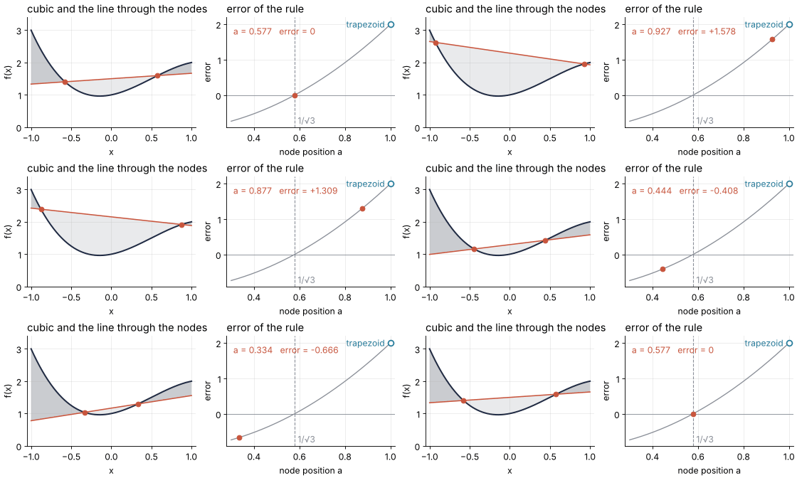
The smallest case shows the mechanism. Put two points on \([-1, 1]\) at \(\pm a\), each with weight 1. The weights add up to 2, the length of the interval, so the constant 1 comes out right. The odd powers \(x\) and \(x^3\) integrate to zero, and the rule gives zero for them too, whatever \(a\) is. That leaves \(x^2\), whose integral is \(2/3\) while the rule gives \(2a^2\). They agree for one value only, \(a = 1/\sqrt3 = 0.57735\).

There is a picture behind this. The estimate \(f(-a) + f(a)\) is the area under the straight line through the two samples, and it is exact when the curve rises above that line by as much area as it sinks below. Here is the cubic \(f(x) = 1 + 0.5x + 1.5x^2 - x^3\), which has all four powers in it, at three settings of \(a\):

Show code

Copy

coef = [1.0, 0.5, 1.5, -1.0]                         # c0 + c1 x + c2 x² + c3 x³
cubic = Polynomial(coef)
exact2 = cubic.integ()(1) - cubic.integ()(-1)
x = np.linspace(-1, 1, 400)

fig, axes = plt.subplots(1, 3, figsize=(8, 2.8), sharey=True)
for ax, a in zip(axes, [1.0, 0.8, 1 / np.sqrt(3)]):
    line = cubic(-a) + (cubic(a) - cubic(-a)) * (x + a) / (2 * a)
    e2 = cubic(-a) + cubic(a) - exact2
    ax.plot(x, cubic(x), color=INK)
    ax.fill_between(x, line, cubic(x), where=cubic(x) >= line, color=MUTED, alpha=0.45, lw=0)
    ax.fill_between(x, line, cubic(x), where=cubic(x) < line, color=MUTED, alpha=0.18, lw=0)
    if a == 1.0:                                     # nodes at the ends: the trapezoid rule, as in the first figure
        ax.plot(x, line, color=SECOND, lw=1.4)
        ax.plot([-a, a], [cubic(-a), cubic(a)], "o", ms=7, mfc="white", mec=SECOND, mew=1.6, zorder=3)
    else:                                            # nodes moved in
        ax.plot(x, line, color=ACCENT, lw=1.4)
        ax.plot([-a, a], [cubic(-a), cubic(a)], "o", color=ACCENT, ms=6, zorder=3)
    shown = "0" if abs(e2) < 1e-12 else f"{e2:+.2f}"
    ax.text(0.5, 0.05, f"a = {a:.3f}, error {shown}", transform=ax.transAxes, ha="center")
    ax.set(xlabel="x", ylim=(0, 3.6))
axes[0].set_ylabel("f(x)")
fig.tight_layout()
plt.show()

At \(a = 1\) the rule is the trapezoid rule and overestimates by 2.00. At \(a = 0.8\) the error is down to 0.92, and at \(a = 1/\sqrt3\) the shaded areas cancel and the error is zero.

Since the odd part of the cubic comes out exact at any \(a\), the error depends on the \(x^2\) coefficient \(c_2\) alone: it is \(2c_2(a^2 - 1/3)\), a parabola in \(a\) with one positive zero. Watch it while the two nodes slide in and back out:

"""Two-point lock: a symmetric two-point rule on a cubic, and its error against the node position a.

Renders ../../assets/two-point-lock.gif. Run it from any directory:

    python scene.py
"""
from pathlib import Path

import numpy as np
import matplotlib.pyplot as plt
from matplotlib.animation import FuncAnimation, PillowWriter
from PIL import Image

OUT = Path(__file__).resolve().parents[2] / "assets" / "two-point-lock.gif"
INK, ACCENT, SECOND, MUTED = "#1f2a44", "#c8553d", "#2a7f9e", "#8a8f98"
plt.rcParams.update({"axes.spines.top": False, "axes.spines.right": False,
                     "axes.grid": True, "grid.alpha": 0.25, "font.size": 11})

# ---- the cubic of the tutorial, and the error of the rule f(-a) + f(a) on it
c0, c1, c2, c3 = 1.0, 0.5, 1.5, -1.0
def f(x):
    return c0 + c1 * x + c2 * x**2 + c3 * x**3
exact = 2 * c0 + 2 * c2 / 3
def error(a):                                   # the odd terms cancel, only x² is left
    return f(-a) + f(a) - exact

a_gauss = 1 / np.sqrt(3)
def ease(a0, a1, n):                            # from a0 to a1 in n frames, slow at both ends
    return a0 + (a1 - a0) * (1 - np.cos(np.linspace(0, np.pi, n, endpoint=False))) / 2
# start and end at the lock, so that the loop has no seam
frames = np.concatenate([np.full(12, a_gauss),               # rest at the lock
                         ease(a_gauss, 1, 22),               # slide out to the trapezoid rule
                         ease(1, 0.3, 40),                   # slide in, past the lock
                         ease(0.3, a_gauss, 22),             # back out to the lock
                         np.full(12, a_gauss)])              # rest there
x = np.linspace(-1, 1, 400)
a_fine = np.linspace(0.3, 1, 300)

# ---- figure, drawn once
fig, (ax1, ax2) = plt.subplots(1, 2, figsize=(7, 2.8), dpi=80, layout="constrained")
ax1.plot(x, f(x), color=INK, lw=1.8)
(chord,) = ax1.plot([], [], color=ACCENT, lw=1.4)
(nodes,) = ax1.plot([], [], "o", color=ACCENT, ms=6)
fills = []
ax1.set(xlim=(-1.05, 1.05), ylim=(0, 3.4), xlabel="x", ylabel="f(x)")
ax1.set_title("cubic and the line through the nodes", loc="left")

ax2.plot(a_fine, error(a_fine), color=MUTED, lw=1.2)
ax2.axvline(a_gauss, color=MUTED, ls="--", lw=1)
ax2.axhline(0, color=MUTED, lw=0.8)
(dot,) = ax2.plot([], [], "o", color=ACCENT, ms=6, zorder=3)
label = ax2.text(0.04, 0.92, "", transform=ax2.transAxes, va="top", color=ACCENT)
ax2.set(xlim=(0.28, 1.02), ylim=(-0.9, 2.2), xlabel="node position a", ylabel="error")
ax2.set_title("error of the rule", loc="left")
ax2.text(a_gauss + 0.015, -0.8, "1/√3", color=MUTED)
# a = 1 puts the nodes at the ends: the trapezoid rule, in its color from the other figures
ax2.plot([1], [error(1)], "o", ms=7, mfc="white", mec=SECOND, mew=1.6, zorder=2)
ax2.text(0.975, error(1), "trapezoid", color=SECOND, ha="right", va="center")

# ---- one frame: a function of the node position alone
def update(a):
    for coll in fills:
        coll.remove()
    fills.clear()
    line = f(-a) + (f(a) - f(-a)) * (x + a) / (2 * a)
    chord.set_data(x, line)
    nodes.set_data([-a, a], [f(-a), f(a)])
    fills.append(ax1.fill_between(x, line, f(x), where=f(x) >= line, color=MUTED, alpha=0.45, lw=0))
    fills.append(ax1.fill_between(x, line, f(x), where=f(x) < line, color=MUTED, alpha=0.18, lw=0))
    e = error(a)
    dot.set_data([a], [e])
    label.set_text(f"a = {a:.3f}   error = " + ("0" if abs(e) < 1e-12 else f"{e:+.3f}"))

# ---- render, and read back what was written
OUT.parent.mkdir(exist_ok=True)
FuncAnimation(fig, update, frames=frames).save(OUT, writer=PillowWriter(fps=12))
plt.close(fig)
with Image.open(OUT) as im:
    delay = im.info["duration"]
    print(f"{OUT.name}: {im.width} x {im.height} px, {im.n_frames} frames at {delay} ms, "
          f"{im.n_frames * delay / 1000:.1f} s, {OUT.stat().st_size / 1024:,.0f} kB")

Two free nodes land on the same answer

The symmetry was an assumption. Drop it and let the two nodes \(x_1 < x_2\) go anywhere in \([-1, 1]\). The weights then follow from the points: requiring \(1\) and \(x\) to come out exact is a linear system with the solution \(w_1 = 2x_2/(x_2 - x_1)\) and \(w_2 = -2x_1/(x_2 - x_1)\). With those weights the error of the rule is \(-2x_1x_2 - 2/3\) on \(x^2\) and \(-2x_1x_2(x_1 + x_2)\) on \(x^3\). The first vanishes on the hyperbola \(x_1 x_2 = -1/3\), the second on the line \(x_1 = -x_2\) and on the two axes. Draw the zero sets in the plane of the two nodes:

Show code

Copy

def weights_two(x1, x2):
    """Weights that make 1 and x exact for nodes x1 < x2 on [-1, 1]."""
    return 2 * x2 / (x2 - x1), -2 * x1 / (x2 - x1)

w1, w2 = weights_two(-1 / np.sqrt(3), 1 / np.sqrt(3))
print(f"weights at ±1/√3: {w1:.6f}, {w2:.6f}")

fig, ax = plt.subplots(figsize=(4.6, 4.6))
ax.plot([-1, 1], [-1, 1], color=MUTED, ls="--", lw=1)             # x₁ = x₂, not a rule
for branch in [np.linspace(-1, -1 / 3, 200), np.linspace(1 / 3, 1, 200)]:
    ax.plot(branch, -1 / (3 * branch), color=INK)              # x² exact
ax.plot([-1, 1], [1, -1], color=INK, lw=1.2)                    # x³ exact: the line and the two axes
ax.axhline(0, color=INK, lw=1.2)
ax.axvline(0, color=INK, lw=1.2)
xg2 = 1 / np.sqrt(3)
ax.plot([-xg2], [xg2], "o", color=ACCENT, ms=7, zorder=4)
ax.annotate("Gauss: ±1/√3", (-xg2, xg2), xytext=(-0.95, 0.93), color=ACCENT)
ax.text(-0.95, 0.06, "x₁x₂ = −1/3\nx² exact", color=INK)
ax.text(0.05, -0.72, "x₁ = −x₂\nx³ exact", color=INK)
ax.text(0.46, 0.63, "x₁ = x₂", color=MUTED, rotation=45, ha="center", va="center")
ax.set(xlabel="x₁", ylabel="x₂", xlim=(-1, 1), ylim=(-1, 1), aspect="equal")
plt.show()

weights at ±1/√3: 1.000000, 1.000000

The curves cross once in the half of the square where \(x_1 < x_2\), at \((-0.57735, 0.57735)\), and the weights there are 1 and 1. That is the only solution, and it is the symmetric pair from before: symmetry is not an assumption the rule needs but a property of its answer.

With \(n\) points the \(2n\) equations are polynomial in the nodes, of degree up to \(2n - 1\), and solving them head-on is hopeless beyond a handful of points. They have an answer all the same, if not a closed form: the nodes are the roots of the Legendre polynomial \(P_n\), which SciPy finds numerically. That is not a coincidence, and the Formalization proves it. The Legendre polynomials are what you get by making \(1, x, x^2, \dots\) orthogonal to each other on \([-1, 1]\), one power at a time, and in electrostatics they carry the angular dependence of the multipole expansion. For two points, \(P_2(x) = (3x^2 - 1)/2\) has its roots at \(\pm 1/\sqrt3\), the crossing above. Here is the family up to \(P_5\):

Show code

Copy

fig, ax = plt.subplots(figsize=(7, 3.4))
for k in range(1, 5):
    ax.plot(x, eval_legendre(k, x), color=MUTED, lw=1.1)
ax.plot(x, eval_legendre(5, x), color=INK)
ax.axhline(0, color=MUTED, lw=0.8)
ax.plot(xg, np.zeros(5), "o", color=ACCENT, ms=6, zorder=4)
for xi in xg[2:]:                                   # the roots at and right of 0, in a clear band
    ax.text(xi, -0.93, f"{xi:.3f}", ha="center", color=ACCENT)
ax.text(0.29, 0.40, "P₅", color=INK, ha="center")
ax.text(-0.45, -0.85, "P₁ to P₄", color=MUTED, ha="center")
ax.set(xlabel="x", ylabel="Pₙ(x)", xlim=(-1.02, 1.02), ylim=(-1.05, 1.05))
plt.show()

The five roots of \(P_5\), at 0, \(\pm0.53847\), and \(\pm0.90618\), are the five Gauss nodes of the first figure mapped back to \([-1, 1]\). The property that matters is orthogonality, \(\int_{-1}^{1} P_m P_n\,dx = 0\) for \(m \neq n\). Each \(P_k\) has degree exactly \(k\), so \(P_0, \dots, P_{n-1}\) build every polynomial of degree below \(n\), the way \(1, x, x^2\) do. \(P_n\) is orthogonal to each of them, and therefore to every combination of them:

The whole proof rests on that line.

Formalization

The Gauss-Legendre rule with \(n\) points is

with \(x_i\) the roots of \(P_n\) and \(w_i = \int_{-1}^{1} \ell_i(x)\,dx\), where \(\ell_i\) is the polynomial of degree \(n - 1\) that is 1 at \(x_i\) and 0 at the other nodes; in closed form, \(w_i = 2/\big((1 - x_i^2)\,P_n'(x_i)^2\big)\). All weights are positive, so no large terms cancel and amplify rounding. scipy.special.roots_legendre(n) returns nodes and weights on \([-1, 1]\). On \([a, b]\) the nodes move to \((a + b)/2 + (b - a)\,x_i/2\) and the weights are multiplied by \((b - a)/2\).

Why degree \(2n - 1\): take a polynomial \(p\) of that degree and divide it by \(P_n\), so that \(p = q P_n + r\) with \(q\) and \(r\) of degree below \(n\). The integral of \(q P_n\) is zero, because \(P_n\) is orthogonal to every polynomial of lower degree. The rule sees \(q P_n\) as zero too, because it samples only at the roots of \(P_n\). What is left is \(r\), and by the definition of the weights the rule gives \(\sum_i w_i\, r(x_i) = \int_{-1}^{1} \sum_i r(x_i)\,\ell_i(x)\,dx\). The sum inside the integral has degree below \(n\) and matches \(r\) at all \(n\) nodes, so it is \(r\) itself.

Two cells check this. The first computes the five weights from the moment equations (\(1\) to \(x^4\) exact), with roots_legendre, and from the closed formula:

# weights from the moment equations: sum_i w_i x_i^k = integral of x^k over [-1, 1], k = 0..4
moments = np.array([(1 - (-1) ** (k + 1)) / (k + 1) for k in range(5)])
w_moments = np.linalg.solve(np.vander(xg, 5, increasing=True).T, moments)
_, w_scipy = roots_legendre(5)
dP5 = (5 * eval_legendre(4, xg) - 5 * xg * eval_legendre(5, xg)) / (1 - xg**2)
w_closed = 2 / ((1 - xg**2) * dP5**2)
for name, wv in [("moment equations", w_moments), ("roots_legendre", w_scipy), ("closed formula", w_closed)]:
    print(f"{name:17s}", "  ".join(f"{wi:.6f}" for wi in wv))

moment equations  0.236927  0.478629  0.568889  0.478629  0.236927
roots_legendre    0.236927  0.478629  0.568889  0.478629  0.236927
closed formula    0.236927  0.478629  0.568889  0.478629  0.236927

The three rows agree to every printed digit: once the nodes are fixed, the weights are not a further choice. The second cell tests exactness on \([0, 1]\), with one random polynomial of each degree, because on \([-1, 1]\) every symmetric rule gets the odd powers right for free:

rng = np.random.default_rng(315)
rules = {"trapezoid": lambda p: trapezoid(p(s5), x=s5),
         "Simpson": lambda p: simpson(p(s5), x=s5),
         "Gauss": lambda p: gauss(p, 0, 1, 5)}
print("degree  " + "".join(f"{name:>11s}" for name in rules))
for degree in range(12):
    p = Polynomial(rng.uniform(-1, 1, degree + 1))
    exact = p.integ()(1) - p.integ()(0)
    print(f"{degree:4d}    " + "".join(f"{abs(rule(p) - exact):11.0e}" for rule in rules.values()))

degree    trapezoid    Simpson      Gauss
   0          0e+00      0e+00      0e+00
   1          0e+00      0e+00      0e+00
   2          4e-03      2e-16      2e-16
   3          1e-02      0e+00      0e+00
   4          2e-02      5e-04      8e-17
   5          4e-02      2e-03      0e+00
   6          6e-02      3e-03      4e-16
   7          7e-02      7e-03      2e-16
   8          3e-02      5e-04      2e-16
   9          9e-02      1e-02      3e-16
  10          3e-02      2e-03      1e-06
  11          1e-02      2e-03      6e-06

The trapezoid rule is exact up to degree 1, Simpson's rule up to 3, Gauss up to 9, and at degree 10 Gauss misses by 1e-6.

For an integrand with \(2n\) continuous derivatives, the error of the \(n\)-point rule on \([a, b]\) is

for some \(\xi\) in \((a, b)\). Three consequences follow.

Analytic integrands: the error falls exponentially. More points do not shrink a step here. They raise the order of the derivative in the error term, and the factorials make the constant collapse: on \([-1, 1]\) it is 8.1e-10 at \(n = 5\) and 1.2e-24 at \(n = 10\). As long as the derivatives of \(f\) grow more slowly than the constant shrinks, which holds for an integrand that is analytic (equal to its Taylor series) on the interval and near it, the error falls exponentially in \(n\). A merely infinitely differentiable integrand still gets an error falling faster than any power of \(n\). Equal spacing falls only as a power, \(n^{-2}\) or \(n^{-4}\).

Kinks and endpoint singularities: move the trouble into a weight function. The error term needs \(f^{(2n)}\), and \(|x - 0.3|\) has no second derivative at 0.3: on that kink Gauss and the trapezoid rule both fall like \(1/n^2\), with 6.8e-3 and 6.3e-3 at ten points. The pendulum integral of the quad tutorial, \(\int_0^{\theta_0} d\theta/\sqrt{\cos\theta - \cos\theta_0}\), is infinite at \(\theta_0\), where \(\cos\theta - \cos\theta_0 \approx \sin\theta_0\,(\theta_0 - \theta)\) is linear in the distance to the end, so the integrand grows like \((\theta_0 - \theta)^{-1/2}\). Doubling \(n\) from 10 to 20 takes Gauss-Legendre only from 4.0e-2 to 2.0e-2. A weight function \(\rho(x)\) in the orthogonality, \(\int \rho\, p_m p_n\,dx = 0\) for \(m \neq n\), defines a family of polynomials, the proof holds with \(\rho\) inside every integral, and the family's roots with their own weights \(w_i\) (not the values \(\rho(x_i)\)) give \(\int \rho\, h\,dx \approx \sum_i w_i\, h(x_i)\), exact for every \(h\) of degree up to \(2n - 1\). For \(\rho = (1 - x)^\alpha (1 + x)^\beta\) the family is the Jacobi polynomials, with nodes and weights from roots_jacobi(n, alpha, beta). Mapped to \([-1, 1]\), the pendulum integrand is \((1 - x)^{-1/2}\) times a smooth \(h\), and with \(\alpha = -1/2\), \(\beta = 0\) five points give 5.8e-9, against 7.6e-2 for Gauss-Legendre. Gauss-Laguerre (\(e^{-x}\) on \([0, \infty)\)) and Gauss-Hermite (\(e^{-x^2}\) on the whole line) are the same idea for infinite intervals.

kink = lambda x: np.abs(x - 0.3)
kink_exact = (1.3**2 + 0.7**2) / 2
print("kink |x - 0.3| on [-1, 1], absolute error")
for n in [5, 10, 20, 40, 80]:
    xe = equal(n, -1, 1)
    print(f"  n = {n:2d}   trapezoid {abs(trapezoid(kink(xe), x=xe) - kink_exact):.1e}"
          f"   Gauss {abs(gauss(kink, -1, 1, n) - kink_exact):.1e}")

theta_exact = np.sqrt(2) * K                          # the θ-integral is √2 K(m)
def h_jacobi(x):
    """The θ-integrand on [-1, 1] with the factor (1 - x)^(-1/2) taken out: smooth."""
    return theta0 / 2 * np.sqrt(1 - x) * f_theta(theta0 * (1 + x) / 2)

print("pendulum θ-form, singular at θ₀, relative error")
for n in [5, 10, 20, 40]:
    xj, wj = roots_jacobi(n, -0.5, 0)
    legendre = abs(gauss(f_theta, 0, theta0, n) - theta_exact) / theta_exact
    jacobi = abs(np.sum(wj * h_jacobi(xj)) - theta_exact) / theta_exact
    print(f"  n = {n:2d}   Gauss-Legendre {legendre:.1e}   Gauss-Jacobi {jacobi:.1e}")

kink |x - 0.3| on [-1, 1], absolute error
  n =  5   trapezoid 6.0e-02   Gauss 2.6e-02
  n = 10   trapezoid 6.3e-03   Gauss 6.8e-03
  n = 20   trapezoid 2.5e-03   Gauss 1.8e-03
  n = 40   trapezoid 6.0e-04   Gauss 4.3e-04
  n = 80   trapezoid 1.5e-04   Gauss 6.3e-05
pendulum θ-form, singular at θ₀, relative error
  n =  5   Gauss-Legendre 7.6e-02   Gauss-Jacobi 5.8e-09
  n = 10   Gauss-Legendre 4.0e-02   Gauss-Jacobi 0.0e+00
  n = 20   Gauss-Legendre 2.0e-02   Gauss-Jacobi 5.1e-16
  n = 40   Gauss-Legendre 1.0e-02   Gauss-Jacobi 5.8e-15

Matching ends: equal spacing is already exponential. The trapezoid rule's error is a series in \(h^2, h^4, \dots\) whose terms are proportional to the differences \(f'(b) - f'(a)\), \(f'''(b) - f'''(a)\), and so on (the Euler-Maclaurin formula). They all vanish, and the error falls exponentially, for an analytic periodic \(f\) over a full period, and for an \(f\) that is mirror symmetric about both ends of the interval. The textbook form, \(K(m) = \int_0^{\pi/2} d\varphi/\sqrt{1 - m\sin^2\varphi}\), is the second case. With five points the trapezoid rule has 5.5e-7 there and Gauss 7.4e-6. Cut the same integrand off at \(\pi/3\) and the ends no longer match: the trapezoid rule falls back to 2.5e-3, while Gauss has 2.2e-8. Equal spacing wins only when the integrand repeats itself across the ends of the interval; on anything else that is smooth, Gauss wins.

for b, exact, label in [(np.pi / 2, K, "[0, π/2], ends match"),
                        (np.pi / 3, ellipkinc(np.pi / 3, m), "[0, π/3], ends do not")]:
    print(label)
    for n in [5, 9]:
        p = equal(n, 0, b)
        print(f"  n = {n}   trapezoid {abs(trapezoid(f_phi(p), x=p) - exact):.1e}"
              f"   Gauss {abs(gauss(f_phi, 0, b, n) - exact):.1e}")

[0, π/2], ends match
  n = 5   trapezoid 5.5e-07   Gauss 7.4e-06
  n = 9   trapezoid 2.9e-13   Gauss 4.3e-10
[0, π/3], ends do not
  n = 5   trapezoid 2.5e-03   Gauss 2.2e-08
  n = 9   trapezoid 6.3e-04   Gauss 3.7e-14

See it in code

The cell below integrates the smooth form of the pendulum integral from the first section with all three rules for a growing number of points and puts the errors on log-log axes. scipy.special.roots_legendre supplies the Gauss nodes and quad gets the last word. NumPy's leggauss returns the same nodes; use it only where SciPy is not available, because roots_legendre has roots_jacobi and the other weighted rules beside it.

Show code

Copy

n_equal = 2 ** np.arange(1, 9) + 1                  # 3, 5, 9, ..., 257: Simpson needs odd n
n_gauss = np.arange(2, 21)
floor = np.finfo(float).eps * K
err_trap = np.array([abs(trapezoid(f_s(equal(n)), x=equal(n)) - K) for n in n_equal])
err_simp = np.array([abs(simpson(f_s(equal(n)), x=equal(n)) - K) for n in n_equal])
err_gauss = np.array([max(abs(gauss(f_s, 0, 1, n) - K), floor / 4) for n in n_gauss])  # 0 cannot go on a log axis

fig, ax = plt.subplots(figsize=(7, 3.8))
ax.loglog(n_equal, err_trap, "o-", color=SECOND, ms=5)
ax.loglog(n_equal, err_simp, "s-", color=SECOND, ms=5)
ax.loglog(n_gauss, err_gauss, "o-", color=ACCENT, ms=5)
ax.axhline(floor, color=MUTED, ls=":", lw=1)
guide = np.array([20, 200])
ax.loglog(guide, 2e-2 * guide**-2.0, color=MUTED, lw=1)          # slope guides, a decade below the data
ax.loglog(guide, 3e-2 * guide**-4.0, color=MUTED, lw=1)
ax.text(235, 2e-2 * 200.0**-2, "n⁻²", color=MUTED, va="center")
ax.text(235, 3e-2 * 200.0**-4, "n⁻⁴", color=MUTED, va="center")
ax.text(300, err_trap[-1], "trapezoid", color=SECOND, va="center")
ax.text(300, err_simp[-1], "Simpson", color=SECOND, va="center")
ax.text(14, 1e-10, "Gauss-Legendre", color=ACCENT)
ax.text(300, floor * 1.6, "rounding", color=MUTED, va="bottom")
ax.set(xlabel="number of points n", ylabel="absolute error", xlim=(1.7, 600), ylim=(5e-17, 1))
plt.show()

for n in [17, 65]:
    i = list(n_equal).index(n)
    print(f"{n} points: trapezoid {err_trap[i]:.1e}, Simpson {err_simp[i]:.1e}, "
          f"Gauss {abs(gauss(f_s, 0, 1, n) - K):.1e}")
x10, w10 = roots_legendre(10)
print(f"leggauss agrees with roots_legendre: {np.allclose(np.polynomial.legendre.leggauss(10), (x10, w10), rtol=0, atol=1e-15)}")
print(f"10-point Gauss alone: error {abs(gauss(f_s, 0, 1, 10) - K):.1e}")
value, estimate, info = quad(f_s, 0, 1, full_output=1)
print(f"quad: {value:.15f} (error {abs(value - K):.0e}), estimate {estimate:.1e}, {info['neval']} evaluations")

17 points: trapezoid 6.5e-04, Simpson 5.8e-06, Gauss 2.2e-16
65 points: trapezoid 4.1e-05, Simpson 2.4e-08, Gauss 0.0e+00
leggauss agrees with roots_legendre: True
10-point Gauss alone: error 2.0e-11
quad: 1.854074677301372 (error 2e-16), estimate 8.8e-13, 21 evaluations

On the log-log axes the trapezoid and Simpson errors lie on straight lines of slope −2 and −4, the textbook rates. The Gauss curve bends downward instead and reaches rounding level by 15 points. At 17 points it is at 2.2e-16, where the trapezoid rule still has 6.5e-4 and Simpson's rule 5.8e-6; the trapezoid rule needs 65 points to get to 4.1e-5.

quad returns \(K\) to every printed digit from 21 evaluations, one pass of a Gauss-Kronrod rule: a 10-point Gauss rule plus 11 points placed by Kronrod so that the 10 Gauss values are reused, together exact to degree 31. QUADPACK, the Fortran library inside quad, starts its error estimate from the difference between the 21-point and the 10-point answers. The 10-point answer is off by 2.0e-11, and since so small a difference means the 21-point answer is far better still, QUADPACK shrinks it to 8.8e-13. The true error is 2e-16: the estimate is cautious by more than three orders of magnitude. That is the error estimate Numerical integration with scipy.integrate reported without saying where it came from.

Where it shows up

• Engineering: finite elements. The stiffness matrix of an element is an integral over the element, and finite element codes evaluate it at 2 × 2 or 3 × 3 Gauss points per quadrilateral, chosen to integrate the products of the element's polynomials exactly. scikit-fem's intorder sets that degree, and integrating with one point fewer on purpose, reduced integration, is the classic cure for the locking of thin elements in bending.
• Physics: spectral methods. Spectral and spectral-element codes collocate a differential equation at Gauss or Gauss-Lobatto nodes, where Lobatto includes the two ends of the interval and pays for them with two degrees of exactness. Chebyshev collocation for eigenvalue problems: a neutron on a mirror uses the Chebyshev relatives of these nodes.
• Chemistry: quantum chemistry. Electron repulsion integrals over Gaussian basis functions are computed by Rys quadrature, a Gauss rule whose weight function is built for the Boys function that appears in them. Density functional programs often integrate the exchange-correlation energy on grids of Gauss-Chebyshev radial points times Lebedev angular points around each atom.
• Statistics: uncertainty propagation. The mean of \(f(X)\) for a normally distributed \(X\) is an integral with the weight \(e^{-x^2}\) after a change of variable, so Gauss-Hermite with \(n\) nodes gets it exactly for any polynomial \(f\) of degree up to \(2n - 1\). For a smooth \(f\) a handful of evaluations replaces the thousands of samples of Uncertainty propagation by sampling with NumPy.
• Physics: scattering theory. The Lippmann-Schwinger equation in momentum space is an integral equation, and putting its integral on a Gauss-Legendre grid turns it into a matrix equation over the nodes. The size of that matrix is the number of nodes, so the exponential convergence of Gauss quadrature is what keeps it small.

In every case the rule from the Formalization carries over: where you may choose the points, put them at the roots of the polynomials orthogonal with your weight function, and the smoothness of what is left decides how fast you converge.

Further reading

• SciPy references for roots_legendre, roots_jacobi, and quad, and NumPy's leggauss.
• Davis and Rabinowitz, Methods of Numerical Integration, for the error terms and the whole family of Gauss rules.
• Trefethen, Approximation Theory and Approximation Practice, the chapter on Clenshaw-Curtis and Gauss quadrature, and his article "Is Gauss quadrature better than Clenshaw-Curtis?" (SIAM Review, 2008).
• Related tutorials on this site: Numerical integration with scipy.integrate: the area under a measured peak; Monte Carlo integration: why the error falls as one over the square root of N, for why every quadrature rule loses in many dimensions; Polynomial roots are eigenvalues: why Wilkinson's polynomial loses its roots, the same trick SciPy uses for the nodes, which it computes as eigenvalues of a tridiagonal matrix; Finite elements: hat functions, the weak form, and a heated bar; and in Julia, Numerical integration with QuadGK.jl: the area under a measured peak.
• Download the notebook. It was executed with the library versions in the header.