Solve recurrences with SymPy's rsolve: fixation in the Moran model
Afterwards you can solve a linear recurrence with boundary values using SymPy's rsolve, handle its degenerate case with limit, and check it by simulation.
- Field
- Biology, Mathematics
- Prerequisites
- Random numbers with numpy.random: ten thousand reproducible random walks, SymPy from the ground up: where the pendulum's 1.74 % comes from, The standard error of the mean: why four times the data halves the error
- Libraries
matplotlib 3.11.2numpy 2.4.3sympy 1.14.0
py-sympy-rsolve.ipynb, executed with the versions above. The download needs a free account
Run it yourself. In a terminal, this installs exactly the versions above:
pip install numpy==2.4.3 sympy==1.14.0 matplotlib==3.11.2 jupyterlabThe problem: how often does a fitter mutant take over?
A mutant that is picked to reproduce 1 % more often than its neighbors appears in a population of \(N = 100\) haploid individuals. How often does its line take over the whole population? The exact answer is 0.0157, against 0.0100 for a mutant without an advantage, and it comes out of a linear recurrence that SymPy's rsolve solves in one call. The model is Moran's: the population changes one event at a time. One individual is picked to reproduce, with probability proportional to its fitness \(r\), one is picked uniformly at random to die, and the offspring takes its place. Sooner or later the mutant's line is lost or fills the population, which is called fixation. The 1 % advantage raises the chance by more than half, and the mutant is still lost 98 times in 100.
Let \(\phi_k\) be the probability of fixation when \(k\) of the \(N\) individuals are mutants. Step 1 shows that it obeys
A recurrence links each value to its neighbors the way an ODE links a function to its derivatives, and SymPy, introduced in SymPy from the ground up, solves one with rsolve as it solves an ODE with dsolve. The boundary values take the place of initial conditions: with no mutant left nothing can fix, and with \(N\) the job is done.

This is where we end up: the chance that one mutant takes over, against its fitness, for three population sizes. The lines are the exact formula from rsolve, the dots 20,000 simulated populations each. Fixation probability by simulation asks the same question for the Wright-Fisher model, which has no exact formula, and Genetic drift covers the neutral case.
Setup
The symbols carry the assumptions that SymPy needs later: \(k\) and \(N\) are integers, \(r\) is positive.
import warnings
import numpy as np
import sympy as sp
import matplotlib.pyplot as plt

plt.rcParams.update({
    "figure.figsize": (7, 3.6), "figure.dpi": 110,
    "axes.spines.top": False, "axes.spines.right": False,
    "axes.grid": True, "grid.alpha": 0.25,
    "font.size": 11, "lines.linewidth": 1.8,
})
INK, ACCENT, SECOND, MUTED = "#1f2a44", "#c8553d", "#2a7f9e", "#8a8f98"

k = sp.symbols("k", integer=True, nonnegative=True)
N = sp.symbols("N", integer=True, positive=True)
r = sp.symbols("r", positive=True)
phi = sp.Function("phi")

rng = np.random.default_rng(414)
R = 20_000          # simulated populations per point

print(f"SymPy {sp.__version__}")
SymPy 1.14.0
Step 1: Write the Moran model as a recurrence
Follow the population through one event, starting from \(k\) mutants. The chance of winning from there depends only on \(k\), not on how the population got to \(k\), so after the event it is the same function \(\phi\) at the new count. The count goes up by one when a mutant reproduces and a wild type dies, down by one in the opposite case, and stays where it is otherwise:
The first factor is who reproduces, weighted by fitness, the second who dies. Averaging over the three outcomes, and then moving the last term to the left,
Divide by \(P_-\) and only the ratio \(P_+/P_-\) is left. SymPy computes it, and the recurrence follows:
P_plus = r * k / (r * k + N - k) * (N - k) / N
P_minus = (N - k) / (r * k + N - k) * k / N
print("P+/P- =", sp.simplify(P_plus / P_minus))

eq = r * phi(k + 1) - (1 + r) * phi(k) + phi(k - 1)
print(eq, "= 0")
P+/P- = r
r*phi(k + 1) - (r + 1)*phi(k) + phi(k - 1) = 0
The ratio is \(r\), whatever \(k\) and \(N\). So \(N\) has dropped out of the recurrence and survives only in the boundary value \(\phi_N = 1\). The same ratio makes the simulation in Step 5 cheap: of the events that change the count, a fraction \(r/(1+r)\) moves it up.
Step 2: Solve it with rsolve and its boundary values
rsolve takes the recurrence as an expression equal to zero, the unknown as phi(k), and the boundary values as a dict keyed by the function at integer points. For \(N = 100\):
sol_100 = sp.rsolve(eq, phi(k), {phi(0): 0, phi(100): 1})
print(sp.simplify(sol_100))
phi1_100 = sol_100.subs({k: 1, r: sp.Rational(101, 100)})
print(f"phi_1 at N = 100, r = 1.01: {float(phi1_100):.7f}")
r**(100 - k)*(r**k - 1)/(r**100 - 1)
phi_1 at N = 100, r = 1.01: 0.0157087
That is the 0.0157 from the opening. A symbolic \(N\) does not go into the dict (Pitfall 2), so for general \(N\) call rsolve without boundary values:
gen = sp.rsolve(eq, phi(k))
print(gen)
print(sorted(gen.free_symbols, key=str))      # a set prints in no fixed order
C0 + C1/r**k
[C0, C1, k, r]
Two constants, as a second-order recurrence needs. To fix them you need them as Python objects. rsolve names them C0 and C1, and a SymPy symbol is identified by its name and its assumptions, nothing else. So symbols made by hand with the same names and no assumptions are the very ones inside the answer. Given a list of equations and a list of unknowns, solve returns a dict from each unknown to its value, which is the form subs takes:
C0, C1 = sp.symbols("C0 C1")
consts = sp.solve([gen.subs(k, 0), gen.subs(k, N) - 1], [C0, C1])
print(consts)
sol = sp.simplify(gen.subs(consts))
print(sol)
print(f"phi_1 at N = 100, r = 1.01: {float(sol.subs({k: 1, N: 100, r: 1.01})):.7f}")
{C0: r**N/(r**N - 1), C1: -r**N/(r**N - 1)}
r**(N - k)*(r**k - 1)/(r**N - 1)
phi_1 at N = 100, r = 1.01: 0.0157087
The general formula reproduces the number. Now check it in the recurrence itself. The obvious subs does not do it:
print("subs:   ", eq.subs(phi(k), sol))
print("replace:", sp.simplify(eq.replace(phi, sp.Lambda(k, sol))))
subs:    r*phi(k + 1) - r**(N - k)*(r + 1)*(r**k - 1)/(r**N - 1) + phi(k - 1)
replace: 0
subs replaced only the term written exactly phi(k) and left phi(k + 1) and phi(k - 1) alone. sp.Lambda(k, sol) is SymPy's anonymous function, the counterpart of Python's lambda, and replace(phi, ...) swaps the function itself for it, so every phi(...) becomes sol at its own argument. The residual is 0.
Step 3: Take the neutral case r = 1 with the characteristic equation and limit
At \(r = 1\) the mutant is neutral, and the formula should give the neutral answer. It does not:
print(sol.subs(r, 1))
nan
Numerator and denominator both vanish. The reason is in the characteristic equation. The trial solution \(\phi_k = x^k\) plays the role \(e^{\lambda t}\) plays for a linear ODE: it turns a shift of \(k\) by one into a multiplication by \(x\). Put it into eq with replace, divide by \(x^{k-1}\), let powsimp merge the powers of \(x\), and the recurrence becomes a quadratic:
x = sp.symbols("x")
char = sp.powsimp(sp.expand(eq.replace(phi, sp.Lambda(k, x**k)) / x**(k - 1)))
print(char, "=", sp.factor(char))
print("roots at r = 1:", sp.roots(char.subs(r, 1), x))
r*x**2 - r*x - x + 1 = (x - 1)*(r*x - 1)
roots at r = 1: {1: 2}
The roots are 1 and \(1/r\), the constant and the \(r^{-k}\) in rsolve's answer. The boundary values fix the constants through \(C_0 + C_1 = 0\) and \(C_0 + C_1 r^{-N} = 1\), so \(C_1 = -1/(1 - r^{-N})\), the \(r^N - 1\) printed in Step 2. At \(r = 1\) the two roots merge, \(1^k\) and \(r^{-k}\) become the same function, and the two conditions ask \(C_0 + C_1\) to be 0 and 1 at once: the denominator is 0. There are two ways out. The limit of the general formula:
print(sp.limit(sol, r, 1))
k/N
Or rsolve at \(r = 1\), with the constants fixed as before:
gen_neutral = sp.rsolve(eq.subs(r, 1), phi(k))
print(gen_neutral)
print(gen_neutral.subs(sp.solve([gen_neutral.subs(k, 0), gen_neutral.subs(k, N) - 1], [C0, C1])))
C0 + C1*k
k/N
The extra factor \(k\) in C0 + C1*k is what a double root brings, as \(t\,e^{\lambda t}\) does for an ODE: a second function that differs from the constant, so the two conditions can be met again. Both routes give \(k/N\): a neutral mutant's chance of fixation is its share of the population, as Genetic drift found for the Wright-Fisher model.
Step 4: Take N to infinity and compare with the diffusion approximation
For one mutant the formula is short, and in a large population you would expect a limit that no longer depends on \(N\). limit refuses to give it:
phi1 = sp.simplify(sol.subs(k, 1))
print("phi_1 =", phi1)
try:
    sp.limit(phi1, N, sp.oo)
except NotImplementedError as err:
    print("NotImplementedError:", err)
phi_1 = r**(N - 1)*(r - 1)/(r**N - 1)
NotImplementedError: Result depends on the sign of sign(log(r))
The power \(r^N\) in the formula grows without bound when \(r > 1\) and goes to 0 when \(r < 1\), so the limit has two answers and SymPy will not pick one. Tell it which case you mean by writing \(r\) through a positive symbol \(s\):
s = sp.symbols("s", positive=True)
print("beneficial, r = 1 + s:  ", sp.limit(phi1.subs(r, 1 + s), N, sp.oo))
print("harmful,    r = 1/(1+s):", sp.limit(phi1.subs(r, 1 / (1 + s)), N, sp.oo))
print(f"1 - 1/r at r = 1.01: {1 - 1 / 1.01:.5f}")
beneficial, r = 1 + s:   s/(s + 1)
harmful,    r = 1/(1+s): 0
1 - 1/r at r = 1.01: 0.00990
For a beneficial mutant the limit is \(s/(1+s) = 1 - 1/r\), 0.0099 at \(r = 1.01\), and for a harmful one it is 0. In a large population the help from drift that lifted \(N = 100\) to 0.0157 is gone, and a harmful mutant never fixes.
Population genetics usually replaces the recurrence by a differential equation in the frequency \(k/N\), the diffusion approximation. Its solution for the Moran model is \(u_k = (1 - e^{-sk})/(1 - e^{-sN})\) with \(s = r - 1\). It is the Moran version of the formula Kimura derived in 1962 for the Wright-Fisher model, which has \(4N_e s\), with \(N_e\) the effective population size, where this one has \(Ns\). The exact result has \(r^{-k}\) where the diffusion formula has \(e^{-sk}\), and the two match if \(r = e^{s}\). To test that, put \(r = e^{\sigma}\) into the exact result and subtract the diffusion formula with \(s = \sigma\):
sigma = sp.symbols("sigma", positive=True)
kimura = (1 - sp.exp(-s * k)) / (1 - sp.exp(-s * N))
print(sp.simplify(sol.subs(r, sp.exp(sigma)) - kimura.subs(s, sigma)))

exact_u1 = sp.lambdify((N, r), phi1)
kimura_u1 = sp.lambdify((N, r), kimura.subs({k: 1, s: r - 1}))
for r_val in (1.01, 1.10):
    e, d = exact_u1(100, r_val), kimura_u1(100, r_val)
    print(f"N = 100, r = {r_val:.2f}: exact {e:.6f}  diffusion {d:.6f}  ({100 * (d / e - 1):+.2f} %)")
0
N = 100, r = 1.01: exact 0.015709  diffusion 0.015741  (+0.21 %)
N = 100, r = 1.10: exact 0.090916  diffusion 0.095167  (+4.68 %)
The difference is 0: the diffusion formula is exact if \(s\) means \(\ln r\). With \(s = r - 1\), as it is usually written, \(u\) for one mutant is 0.21 % high at \(r = 1.01\) and 4.7 % high at \(r = 1.10\). The two numeric functions come from lambdify, as in Derive a Jacobian with SymPy and pass it to solve_ivp with lambdify.
Step 5: Simulate the Moran model and draw the figure
From Step 1, only the events that change the count matter for who wins, and given a change the count goes up with probability \(r/(1+r)\). So each population is a random walk of steps of plus or minus one, started at \(k = 1\). np.cumsum of a row of steps gives the count after each step, the walk's path, and argmax on (path <= 0) | (path >= N) finds the first hit of 0 or \(N\), once any has confirmed that there is a hit at all. Steps are drawn in blocks; a population that has hit neither end by the end of a block continues from its last count in the next one.
def fixation(N, r):
    """Fraction of R walks from 1 that reach N before 0, and its standard error."""
    p_up = r / (1 + r)
    count = np.ones(R, dtype=np.int64)
    fixed = np.zeros(R, dtype=bool)
    still_open = np.arange(R)
    while still_open.size:
        block = min(1 << 16, max(256, (1 << 22) // still_open.size))   # a few million steps per draw
        steps = np.where(rng.random((still_open.size, block)) < p_up, 1, -1)
        path = count[still_open, None] + np.cumsum(steps, axis=1)
        hit = (path <= 0) | (path >= N)
        done = hit.any(axis=1)
        first = hit.argmax(axis=1)
        fixed[still_open[done]] = path[done, first[done]] >= N
        count[still_open[~done]] = path[~done, -1]
        still_open = still_open[~done]
    u = fixed.mean()
    return u, np.sqrt(u * (1 - u) / R)

r_sim = [0.96, 0.98, 1.00, 1.01, 1.02, 1.04, 1.06, 1.08, 1.10]
results = {}
print("   N     r   simulated            exact     distance")
for N_val in (10, 100, 1000):
    for r_val in r_sim:
        exact = 1 / N_val if r_val == 1 else exact_u1(N_val, r_val)
        if R * exact < 50:                  # too few fixations to estimate
            continue
        u, se = fixation(N_val, r_val)
        results[N_val, r_val] = (u, se)
        print(f"{N_val:4d}  {r_val:.2f}   {u:.5f} ± {se:.5f}   {exact:.5f}   {(u - exact) / se:+5.1f} se")
   N     r   simulated            exact     distance
  10  0.96   0.08300 ± 0.00195   0.08265    +0.2 se
  10  0.98   0.09245 ± 0.00205   0.09116    +0.6 se
  10  1.00   0.09850 ± 0.00211   0.10000    -0.7 se
  10  1.01   0.10415 ± 0.00216   0.10454    -0.2 se
  10  1.02   0.10945 ± 0.00221   0.10914    +0.1 se
  10  1.04   0.11585 ± 0.00226   0.11855    -1.2 se
  10  1.06   0.12735 ± 0.00236   0.12818    -0.4 se
  10  1.08   0.13580 ± 0.00242   0.13799    -0.9 se
  10  1.10   0.14710 ± 0.00250   0.14795    -0.3 se
 100  0.98   0.00355 ± 0.00042   0.00312    +1.0 se
 100  1.00   0.00980 ± 0.00070   0.01000    -0.3 se
 100  1.01   0.01520 ± 0.00087   0.01571    -0.6 se
 100  1.02   0.02065 ± 0.00101   0.02275    -2.1 se
 100  1.04   0.03810 ± 0.00135   0.03924    -0.8 se
 100  1.06   0.05615 ± 0.00163   0.05677    -0.4 se
 100  1.08   0.07315 ± 0.00184   0.07411    -0.5 se
 100  1.10   0.09415 ± 0.00207   0.09092    +1.6 se
1000  1.01   0.01055 ± 0.00072   0.00990    +0.9 se
1000  1.02   0.02025 ± 0.00100   0.01961    +0.6 se
1000  1.04   0.03935 ± 0.00137   0.03846    +0.6 se
1000  1.06   0.05775 ± 0.00165   0.05660    +0.7 se
1000  1.08   0.07530 ± 0.00187   0.07407    +0.7 se
1000  1.10   0.08845 ± 0.00201   0.09091    -1.2 se
r_grid = np.linspace(0.96, 1.10, 300)     # steps around r = 1 exactly (Pitfall 3)
fig, ax = plt.subplots(figsize=(7, 4))
for N_val, alpha, (x_lab, y_lab, ha) in [(10, 1.0, (0.962, 0.115, "left")), (100, 0.65, (0.962, 8e-3, "left")),
                                          (1000, 0.4, (0.9975, 6.5e-4, "right"))]:
    ax.plot(r_grid, exact_u1(N_val, r_grid), color=INK, alpha=alpha)
    ax.text(x_lab, y_lab, f"N = {N_val}", color=INK, alpha=max(alpha, 0.6), ha=ha)
    pts = [(rv, *results[N_val, rv]) for rv in r_sim if (N_val, rv) in results]
    rv, u, se = np.array(pts).T
    ax.errorbar(rv, u, yerr=2 * se, fmt="o", ms=4, capsize=2, lw=1, color=ACCENT)
r_big = r_grid[r_grid > 1]
ax.plot(r_big, 1 - 1 / r_big, color=MUTED, ls="--", lw=1)
ax.text(1.004, 6.5e-4, "N → ∞", color=MUTED)                      # beside the dashed line where it shows
ax.axvline(1, color=SECOND, lw=1)
ax.text(1.0015, 0.25, "neutral, r = 1", color=SECOND)
ax.set(xlabel="fitness of the mutant, r", ylabel="fixation probability of one mutant, φ₁",
       yscale="log", xlim=(0.956, 1.104), ylim=(5e-4, 0.4))
plt.show()
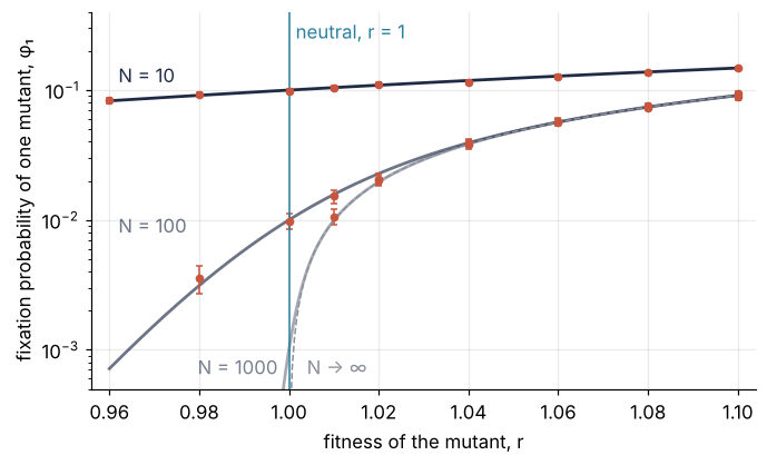
Twenty-two of the 23 points lie within 2 standard errors of the exact value, and the one outside, \(N = 100\) at \(r = 1.02\), misses by 2.1. One in twenty beyond 2 is what chance delivers, so that is agreement. At \(N = 100\) and \(r = 1.01\) the simulation gives 0.0152 ± 0.0009 against the exact 0.0157.
The vertical line marks the neutral mutant, where every curve passes through \(1/N\). At \(N = 10\) a mutant 4 % less fit still fixes: the simulation gives 0.083 at \(r = 0.96\), where the large population of Step 4 gives 0. Above \(r \approx 1.05\) the curves for 100 and 1000 lie on the dashed limit \(1 - 1/r\), and only the small population still feels drift.
Pitfalls
rsolve gives up silently. For a recurrence it cannot solve, rsolve raises no error. It returns None, or an answer with too few constants:
print(sp.rsolve(phi(k + 1) - phi(k) - 1 / k, phi(k)))
print(sp.rsolve((k + 1) * phi(k + 1) - (2 * k + 1) * phi(k) + k * phi(k - 1), phi(k)))
None
C0
The first has the harmonic numbers \(1 + 1/2 + \dots + 1/(k-1)\), plus a constant, as its solution, and the second is of second order and has one constant where it needs two. Test the result for None, count its constants against the order, and substitute it back with replace as in Step 2. This is where frequency-dependent fitness leads; see Variations.
Boundary values with a symbolic index, or as equations. Both look natural and both fail:
for values in ({phi(0): 0, phi(N): 1}, [sp.Eq(phi(0), 0), sp.Eq(phi(100), 1)]):
    try:
        sp.rsolve(eq, phi(k), values)
    except TypeError as err:
        print("TypeError:", err)
TypeError: Cannot convert symbols to int
TypeError: unsupported operand type(s) for -: 'Add' and 'Equality'
Integer keys, {0: 0, 100: 1}, and a plain list of values from \(k = 0\) on work as well as phi(0) and phi(100). What fails are a symbolic index and a list of equations. For a symbolic \(N\), solve for C0 and C1 as in Step 2.
The formula at r = 1 in NumPy. The lambdified formula on a grid that contains 1.0 returns nan there, with a warning:
with warnings.catch_warnings(record=True) as caught:
    warnings.simplefilter("always")
    print(exact_u1(100, np.array([0.99, 1.00, 1.01])))
print(caught[0].category.__name__, caught[0].message)
[0.005832          nan 0.01570866]
RuntimeWarning invalid value encountered in divide
It is the 0/0 of Step 3. np.where(r_grid == 1, 1 / N, ...) fills in the limit but still evaluates the 0/0 and still warns. A grid that steps around 1, as the figure uses, avoids both.
Variations
- Gambler's ruin. Win each game with probability \(p = 0.49\), start with 10 of 20 coins: the same recurrence with \(p\) and \(1 - p\), and
rsolvewith{phi(0): 1, phi(20): 0}gives a ruin probability of 0.5987. - Expected number of games until ruin. Add 1 to the recurrence, which makes it inhomogeneous (a term without \(\phi\)), with \(\phi_0 = \phi_{20} = 0\): 98.7 games from 10 coins.
- Fibonacci and Binet's formula.
phi(k + 2) - phi(k + 1) - phi(k)with{phi(0): 0, phi(1): 1}returns the closed form in \((1 \pm \sqrt 5)/2\). - Frequency-dependent fitness. The ratios \(\gamma_k = P_-/P_+\), down over up, then depend on \(k\),
rsolvemay give up (Pitfall 1), and the classical product formula for a birth-death chain, \(\phi_1 = 1/\bigl(1 + \sum_{j=1}^{N-1} \prod_{i=1}^{j} \gamma_i\bigr)\), takes over. The simulation still works, one event at a time per open population, going up with probability \(P_+/(P_+ + P_-)\) at its current \(k\).
Cheat sheet
phi = sp.Function("phi")
eq = r * phi(k + 1) - (1 + r) * phi(k) + phi(k - 1)        # an expression equal to zero
sp.rsolve(eq, phi(k), {phi(0): 0, phi(100): 1})            # boundary values at integer points only
gen = sp.rsolve(eq, phi(k))                                # general solution in C0, C1
C0, C1 = sp.symbols("C0 C1")                               # same name, no assumptions: same symbols
sol = gen.subs(sp.solve([gen.subs(k, 0), gen.subs(k, N) - 1], [C0, C1]))
assert gen is not None and len(gen.free_symbols & {C0, C1}) == 2   # rsolve gives up silently
sp.simplify(eq.replace(phi, sp.Lambda(k, sol)))            # 0 if sol solves eq; subs is not enough
sp.limit(sol, r, 1)                                        # at a double root of the characteristic equation
Further reading
- SymPy's recurrence solvers, the reference for
rsolveand the special solvers it calls. - Martin A. Nowak, Evolutionary Dynamics: Exploring the Equations of Life (Harvard University Press, 2006), for the Moran process and the product formula.
- P. A. P. Moran, "Random processes in genetics", Proceedings of the Cambridge Philosophical Society 54, 60 to 71 (1958), the original model.
- Warren J. Ewens, Mathematical Population Genetics I (Springer, 2004), for the diffusion approximation.
- Related tutorials on this site: SymPy from the ground up, Derive a Jacobian with SymPy and pass it to solve_ivp with lambdify, Fixation probability by simulation, Genetic drift, The standard error of the mean, Branching processes.
- Download the notebook. It was executed with the library versions in the header.