Change point detection with ruptures: the year the Nile's flow dropped

The problem: when did the Nile's flow drop?

Here are a hundred years of the Nile: the annual flow at Aswan from 1871 to 1970, in units of 10⁸ m³. Until the end of the 1890s the river carried about 1100 a year, afterwards about 850. A drop of 250 is hard to see when the flow scatters by about 130 from one year to the next. Which year did the level change, and is the change real or a run of dry years? Finding that year is change point detection, and ruptures is the Python library for it.

The start of the Aswan dam works in 1898 is the usual explanation. The same question comes with the water level in a well after a new pumping station opens and with the grain size along a sediment core, and a biologist meets it in a fish count below a new dam. In each case you split the record into stretches of constant mean and let the data say how many there are. Finding a split is easy. Deciding that it is more than noise is the work.

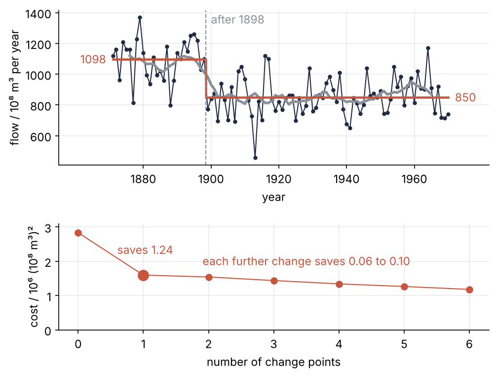
Top: annual Nile flow at Aswan, 1871 to 1970, in 10⁸ m³, with an 11-year moving average and the two segment means, 1098 and 850, as a step after 1898. Bottom: total cost against the number of change points, 0 to 6; it drops by almost half at one change and then barely moves.

The top panel is the record with the change ruptures finds, after 1898, and the two means drawn as a step over an 11-year moving average. The bottom panel is the cost of the best fit for each number of change points: it falls by almost half with the first change and barely moves after that. Step 6 draws this figure.

Setup

statsmodels ships the record as statsmodels.datasets.nile, a table of 100 rows with the year and the flow in 10⁸ m³ per year, so nothing is downloaded. Its description names G. W. Cobb's paper in Biometrika of 1978 as the first analysis of these numbers. The table arrives as a pandas DataFrame, and everything below needs only its two columns as NumPy arrays.

import numpy as np
import matplotlib.pyplot as plt
import ruptures as rpt
import statsmodels.api as sm

plt.rcParams.update({
    "figure.figsize": (7, 3.6), "figure.dpi": 110,
    "axes.spines.top": False, "axes.spines.right": False,
    "axes.grid": True, "grid.alpha": 0.25,
    "font.size": 11, "lines.linewidth": 1.8,
})
INK, ACCENT, SECOND, MUTED = "#1f2a44", "#c8553d", "#2a7f9e", "#8a8f98"

nile = sm.datasets.nile.load_pandas().data
year = nile["year"].to_numpy().astype(int)
flow = nile["volume"].to_numpy(dtype=float)     # 10⁸ m³ per year
n = flow.size

print(f"{n} years from {year[0]} to {year[-1]}, mean {flow.mean():.0f}, "
      f"standard deviation {flow.std(ddof=1):.0f} (10⁸ m³ per year)")

100 years from 1871 to 1970, mean 919, standard deviation 169 (10⁸ m³ per year)

Step 1: Look at the record and its moving average

The first thing anyone does with a noisy record is smooth it. Take a centered 11-year moving average, and for comparison a trailing one, the mean of the ten years up to and including each year:

ma = np.convolve(flow, np.ones(11) / 11, mode="valid")      # centered: years 1876 to 1965
ma_year = year[5:-5]
trail = np.convolve(flow, np.ones(10) / 10, mode="valid")   # trailing: years 1880 to 1970
trail_year = year[9:]

fig, ax = plt.subplots(figsize=(7, 3.2))
ax.plot(year, flow, "o-", color=INK, ms=3, lw=1)
ax.plot(ma_year, ma, color=MUTED, lw=2.5)
ax.hlines(flow.mean(), year[0], year[-1], color=MUTED, lw=1)
ax.text(1972, flow.mean() + 25, f"mean {flow.mean():.0f}", color=MUTED, va="center")
ax.text(1972, ma[-1] - 70, "11-year\naverage", color=MUTED, va="center")
ax.set(xlabel="year", ylabel="flow / 10⁸ m³ per year", xlim=(1866, 1992),
       xticks=range(1880, 1961, 20))
plt.show()

for y in (1894, 1898, 1902):
    print(f"centered 11-year average at {y}: {ma[ma_year == y][0]:5.0f}")
print("first year below the overall mean:",
      "centered", ma_year[np.argmax(ma < flow.mean())],
      "| trailing", trail_year[np.argmax(trail < flow.mean())])

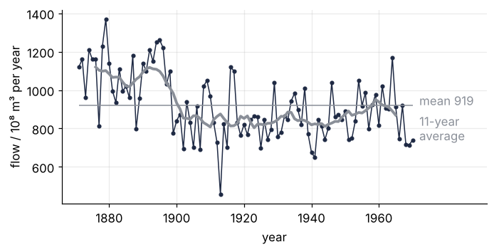
Annual Nile flow at Aswan, 1871 to 1970, in 10⁸ m³, with a centered 11-year moving average and the overall mean of 919. The average slides from about 1100 to about 850 over roughly a decade around 1900.

centered 11-year average at 1894:  1108
centered 11-year average at 1898:  1012
centered 11-year average at 1902:   854
first year below the overall mean: centered 1901 | trailing 1905

The smoother turns a step into a ramp: 1108 in 1894, 1012 in 1898, 854 in 1902, eight years to get down. The two smoothers cross the overall mean four years apart, in 1901 and 1905, and neither crossing is the year the level changed. What you want instead is to split the record into segments with a constant mean each and find the best place for the split.

Step 2: Find the best single split with Dynp

To score a split, ruptures needs a cost for each segment. The l2 cost is the sum of squared deviations of the values from the segment's own mean, and the best split is the one with the smallest total. rpt.Dynp finds it exactly, by dynamic programming, once you tell it how many changes to look for:

algo = rpt.Dynp(model="l2", min_size=2, jump=1).fit(flow)
bkps = algo.predict(n_bkps=1)
print(bkps)
print(f"{year[0]} to {year[bkps[0] - 1]}: mean {flow[:bkps[0]].mean():7.2f}")
print(f"{year[bkps[0]]} to {year[-1]}: mean {flow[bkps[0]:].mean():7.2f}")

[28, 100]
1871 to 1898: mean 1097.75
1899 to 1970: mean  849.97

min_size is the shortest segment allowed, jump the spacing of the candidate split positions. Each number in the result is the end of a segment, exclusive, and the last is always the length of the record. So flow[:28] is 1871 to 1898, and the new level starts at year[28], 1899: about 1098 before, 850 after.

The defaults are not harmless:

print(rpt.Dynp(model="l2").fit(flow).predict(n_bkps=1))

[30, 100]

With jump=5 ruptures tries only every fifth index, and the new level starts in 1901, two years late. Set jump=1 for any record short enough to afford it.

Step 3: Watch the cost fall with every added change

Dynp needs the number of changes, which is the thing you do not know. Ask it for one to six changes and compare the total costs. algo.cost.sum_of_costs takes a list of breakpoints, and a list holding only the length, [100], is the record without a change:

costs = [algo.cost.sum_of_costs([n])]
for k in range(1, 7):
    costs.append(algo.cost.sum_of_costs(algo.predict(n_bkps=k)))

for k, c in enumerate(costs):
    saving = f"saves {costs[k - 1] - c:.2e}" if k else ""
    print(f"{k} changes   cost {c:.3e}   {saving}")
for k in (2, 3):
    ends = np.array(algo.predict(n_bkps=k)[:-1])
    print(f"best with {k} changes: after {year[ends - 1]}")

0 changes   cost 2.835e+06   
1 changes   cost 1.597e+06   saves 1.24e+06
2 changes   cost 1.542e+06   saves 5.51e+04
3 changes   cost 1.438e+06   saves 1.04e+05
4 changes   cost 1.342e+06   saves 9.63e+04
5 changes   cost 1.265e+06   saves 7.71e+04
6 changes   cost 1.181e+06   saves 8.41e+04
best with 2 changes: after [1889 1898]
best with 3 changes: after [1898 1953 1965]

The first change saves 1.24 × 10⁶, every further one between 0.55 and 1.04 × 10⁵, more than ten times less. The best answer with two changes adds a break after 1889; the best with three drops it and puts breaks after 1953 and 1965 instead. The extra breaks jump around. The cost falls with every change you allow, so it cannot stop on its own: how large must a saving be before it is more than noise?

Step 4: Choose the penalty with Pelt

rpt.Pelt minimizes the cost plus a price pen per change, so it accepts a change only if it saves more than pen. The price should be a saving pure noise rarely reaches.

First, the noise level σ, measured without knowing where the change is: the median absolute difference of neighboring years, divided by 0.6745√2. Differences remove the level, and the step spoils only one of the 99, which the median ignores. A difference of two independent values has variance 2σ², and the median absolute value of normal noise is 0.6745σ.

Second, what noise saves. A split after k values replaces one mean by two and lowers the cost by \(S_k^2\,n/(k(n-k))\), with \(S_k\) the sum of the first k deviations from the overall mean: the further the first stretch sits from the rest, the larger the saving. On noise, a place chosen in advance saves σ² on average and the best of all places only a few times more, because neighboring splits cut almost the same noise. The cell sets the price at 2σ² ln n and counts how often noise beats it:

def noise_sigma(z):
    return np.median(np.abs(np.diff(z))) / (0.6745 * np.sqrt(2))

sigma = noise_sigma(flow)
pen = 2 * sigma**2 * np.log(n)
pelt = rpt.Pelt(model="l2", min_size=2, jump=1).fit(flow)
print(f"sigma = {sigma:.0f}, pen = {pen:.3g}, breakpoints {pelt.predict(pen=pen)}")

noise = np.random.default_rng(263).normal(size=(2000, n))     # sigma = 1
S = np.cumsum(noise - noise.mean(axis=1, keepdims=True), axis=1)
k = np.arange(2, n - 1)                                         # min_size=2 at both ends
best = np.max(S[:, k - 1]**2 * n / (k * (n - k)), axis=1)
print(f"best split of noise saves {best.mean():.1f} sigma² on average, "
      f"more than 2 ln n = {2 * np.log(n):.1f} in {100 * np.mean(best > 2 * np.log(n)):.1f} % of 2000 series")

sigma = 115, pen = 1.22e+05, breakpoints [28, 100]
best split of noise saves 4.5 sigma² on average, more than 2 ln n = 9.2 in 5.0 % of 2000 series

σ is 115 and the price 1.22 × 10⁵. The best split of noise saves 4.5σ² on average and beats the price in 5 % of the series, one false split in twenty at n = 100, fewer for longer records. Step 3's later savings, at most 1.04 × 10⁵, fall below it, the first change's 1.24 × 10⁶ is ten times above, and Pelt returns [28, 100] like Dynp. Sweep the penalty and watch the count:

pens = np.geomspace(1e4, 3e6, 60)
counts = np.array([len(pelt.predict(pen=p)) - 1 for p in pens])
for i in np.r_[0, np.flatnonzero(np.diff(counts)) + 1]:
    print(f"pen from {pens[i]:.2e}: {counts[i]:2d} changes")

pen from 1.00e+04: 27 changes
pen from 1.10e+04: 25 changes
pen from 1.34e+04: 23 changes
pen from 1.47e+04: 22 changes
pen from 1.62e+04: 21 changes
pen from 1.79e+04: 20 changes
pen from 1.97e+04: 19 changes
pen from 2.17e+04: 17 changes
pen from 2.39e+04: 16 changes
pen from 2.63e+04: 15 changes
pen from 2.90e+04: 14 changes
pen from 3.51e+04: 11 changes
pen from 4.26e+04: 10 changes
pen from 5.70e+04:  9 changes
pen from 7.62e+04:  7 changes
pen from 8.39e+04:  4 changes
pen from 9.24e+04:  1 changes
pen from 1.26e+06:  0 changes

At 10⁴ there are 27 changes, at 0.84 × 10⁵ still four, from 0.92 × 10⁵ to at least 1.14 × 10⁶ exactly one: a plateau more than a factor of ten wide, with the derived penalty on it.

Step 5: Check every segment with a CUSUM chart

The cumulative sum of deviations from the overall mean, the CUSUM, climbs while the flow is above the mean and falls once it is below. Its peak marks the split:

bkps = pelt.predict(pen=pen)
S = np.cumsum(flow - flow.mean())
k = np.argmax(np.abs(S))

fig, ax = plt.subplots(figsize=(7, 2.8))
ax.plot(year, S, color=INK)
ax.axhline(0, color=MUTED, lw=1)
ax.axvline(year[k], color=MUTED, lw=1, ls="--")
ax.annotate(f"peak {S[k]:.0f} in {year[k]}", (year[k], S[k]), xytext=(12, -6),
            textcoords="offset points", color=INK)
ax.set(xlabel="year", ylabel="cumulative deviation / 10⁸ m³")
plt.show()
print(f"peak {S[k]:.0f} at index {k}, the year {year[k]}")

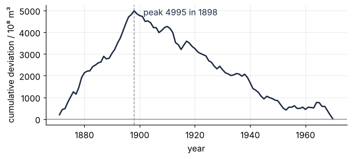
Cumulative sum of deviations of the Nile flow from its mean, in 10⁸ m³, against year. It climbs to a peak of 4995 in 1898, marked by a dashed line, and falls steadily to zero by 1970.

peak 4995 at index 27, the year 1898

The peak sits at 1898, the split ruptures found. To check each segment, divide its largest CUSUM excursion by σ√m, because a sum of m noise values wanders about that far. For a stretch without a change the ratio stays below about 1.36 in 19 cases of 20, the 95 % point of the Kolmogorov distribution:

def cusum_ratio(z, sigma):
    S = np.cumsum(z - z.mean())
    return np.abs(S).max() / (sigma * np.sqrt(z.size))

starts = [0] + bkps[:-1]
print(f"whole record   {cusum_ratio(flow, sigma):.2f}")
for a, b in zip(starts, bkps):
    print(f"{year[a]} to {year[b - 1]}   {cusum_ratio(flow[a:b], sigma):.2f}")

whole record   4.33
1871 to 1898   0.95
1899 to 1970   0.82

The whole record scores 4.33, the two segments 0.95 and 0.82: the split explains the record, and neither segment hides a second change. With more breakpoints the loop simply runs over more segments.

The residuals around the fitted means give two more numbers. One is the drop with its standard error, from the standard deviation s pooled over the segments. The other is the lag-1 autocorrelation, the correlation of each residual with the next, which says whether neighboring years are independent:

lengths = np.diff([0] + bkps)
means = np.array([flow[a:b].mean() for a, b in zip(starts, bkps)])
resid = flow - np.repeat(means, lengths)
s = np.sqrt(np.sum(resid**2) / (n - means.size))           # pooled over the segments
se = s * np.sqrt(np.sum(1 / lengths))
rho = np.corrcoef(resid[:-1], resid[1:])[0, 1]
print(f"drop {means[0] - means[1]:.0f} ± {se:.0f}, {(means[0] - means[1]) / se:.1f} standard errors; "
      f"s = {s:.0f}, lag-1 autocorrelation {rho:.2f}")

drop 248 ± 28, 8.7 standard errors; s = 128, lag-1 autocorrelation 0.16

The drop is 248 ± 28, 8.7 standard errors, and that overstates the evidence: the best of 99 candidate splits always looks better than one chosen in advance (multiple testing). The pooled s of 128 is larger than the σ of 115 from Step 4 because neighboring residuals correlate at 0.16. A difference of two values with correlation ρ has variance 2σ²(1 − ρ) instead of 2σ², so σ from differences comes out smaller by √(1 − ρ), and 128 × √0.84 is 117.

Step 6: Test the detector on series with known changes

Generate series from the fitted segments, np.repeat(means, lengths) plus Gaussian noise with the pooled s, and run the whole procedure of Step 4 on each. Then do the same on series of pure noise, where any change found is a false alarm:

def detect(z):
    pen_z = 2 * noise_sigma(z)**2 * np.log(z.size)
    return rpt.Pelt(model="l2", min_size=2, jump=1).fit(z).predict(pen=pen_z)

rng = np.random.default_rng(263)
n_sim = 200
hit = near = 0
for _ in range(n_sim):
    found = detect(np.repeat(means, lengths) + rng.normal(0, s, n))
    if len(found) == len(bkps):
        hit += 1
        near += np.all(np.abs(np.array(found) - bkps) <= 2)     # every break within two years

alarm = cusum_alarm = 0
for _ in range(n_sim):
    z = rng.normal(0, s, n)
    alarm += len(detect(z)) > 1
    cusum_alarm += cusum_ratio(z, noise_sigma(z)) > 1.36

print(f"Nile-like series: right number of changes {hit / n_sim:.2f}, all within two years {near / n_sim:.2f}")
print(f"pure noise:       Pelt finds a change {alarm / n_sim:.2f}, CUSUM ratio above 1.36 {cusum_alarm / n_sim:.2f}")

Nile-like series: right number of changes 0.88, all within two years 0.81
pure noise:       Pelt finds a change 0.08, CUSUM ratio above 1.36 0.03

With this noise and this drop, the detector finds the one change 88 % of the time and invents one in 8 % of the noise series, about one in twelve; Step 4's 5 % counted only the best single split, with σ known. The Nile's change is not noise, and its year is good to a couple of years, not to one. The CUSUM threshold holds as promised, 3 % against the nominal 5 %. For a record of your own with several changes, detect and the generator run unchanged on its bkps.

fig, (ax, ax2) = plt.subplots(2, 1, figsize=(7.5, 5.6), height_ratios=[3.2, 2.2],
                              gridspec_kw={"hspace": 0.45})
ax.plot(year, flow, "o-", color=INK, ms=3, lw=1)
ax.plot(ma_year, ma, color=MUTED, lw=2.5)
ax.step(year, np.repeat(means, lengths), where="mid", color=ACCENT, lw=2.2)
ax.axvline(year[bkps[0]] - 0.5, color=MUTED, lw=1, ls="--")
ax.text(1869, means[0], f"{means[0]:.0f}", color=ACCENT, ha="right", va="center")
ax.text(1972, means[1], f"{means[1]:.0f}", color=ACCENT, va="center")
ax.text(year[bkps[0]] + 1, 1330, f"after {year[bkps[0] - 1]}", color=MUTED)
ax.set(xlabel="year", ylabel="flow / 10⁸ m³ per year", xlim=(1855, 1982),
       xticks=range(1880, 1961, 20))

ax2.plot(range(7), np.array(costs) / 1e6, "o-", color=ACCENT, ms=6, lw=1)
ax2.plot(1, costs[1] / 1e6, "o", color=ACCENT, ms=10)
saves = -np.diff(costs) / 1e6
ax2.text(0.6, (costs[0] + costs[1]) / 2e6, f"saves {saves[0]:.2f}", color=ACCENT)
ax2.text(3.5, costs[3] / 1e6 + 0.45, f"each further change saves {saves[1:].min():.2f} to {saves[1:].max():.2f}",
         color=ACCENT, ha="center")
ax2.set(xlabel="number of change points", ylabel="cost / 10⁶ (10⁸ m³)²", ylim=(0, 3.1))
plt.show()

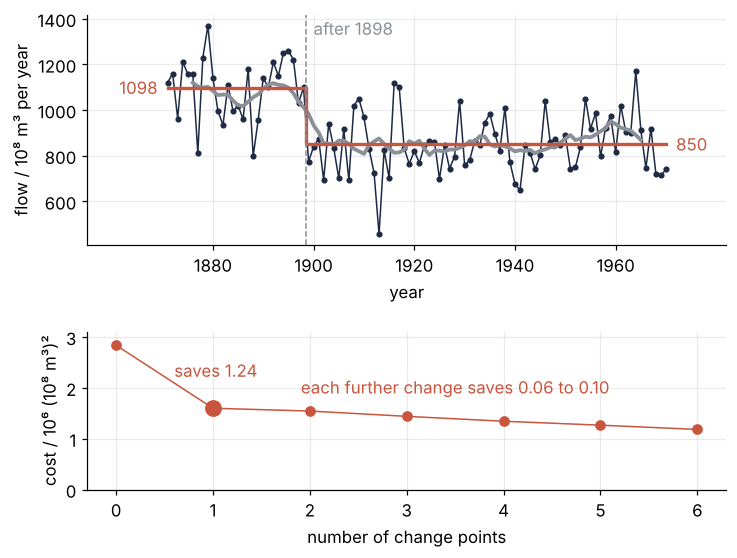
Top: annual Nile flow at Aswan, 1871 to 1970, in 10⁸ m³, with the 11-year moving average and the two segment means, 1098 and 850, as a step after 1898. Bottom: total l2 cost against the number of change points, 0 to 6; the first change cuts it by almost half, later ones barely move it.

One change, after 1898, from 1098 to 850.

Pitfalls

A penalty in the wrong units. The penalty that worked on one record finds nothing, or a change every two years, on another. The cost is in squared units of the data, so the penalty is too. Express the Nile in km³ instead of 10⁸ m³, a factor of ten, and the cost shrinks a hundredfold:

print(rpt.Pelt(model="l2", min_size=2, jump=1).fit(flow / 10).predict(pen=pen))

[100]

The Nile's own penalty now finds no change at all. Never copy a penalty from another record or from a paper; derive it from σ on the record at hand, every time.

The cost model changes the answer. model="rbf" compares values through a kernel, a function that says how alike two values are on a scale from 0 to 1, and looks for any change in the distribution, not only in the mean. Its cost has no units of flow, so the flow penalty means nothing to it:

for p in (1, 2, 5):
    found = rpt.Pelt(model="rbf", min_size=2, jump=1).fit(flow).predict(pen=p)
    print(f"rbf, pen = {p}: {len(found) - 1:2d} changes, breakpoints {found[:3]} ...")

rbf, pen = 1: 12 changes, breakpoints [10, 19, 28] ...
rbf, pen = 2:  1 changes, breakpoints [28, 100] ...
rbf, pen = 5:  1 changes, breakpoints [28, 100] ...

At pen=1 it finds 12 changes, at 2 to 5 the single one at index 28. Pick the cost for the change you mean, l2 for a shift in level, and choose its penalty on its own scale.

Autocorrelated noise produces false changes. On noise where each year remembers 60 % of the last, an AR(1) process with ρ = 0.6, the Step 4 penalty reports changes almost every time. Correlated years drift together and look like short level shifts (see autocorrelation), and the σ from differences comes out too small, for the reason given in Step 5:

rng = np.random.default_rng(263)
plain = inflated = 0
for _ in range(100):
    e = rng.normal(0, s * np.sqrt(1 - 0.6**2), n + 50)
    z = np.zeros(n + 50)
    for t in range(1, n + 50):
        z[t] = 0.6 * z[t - 1] + e[t]
    z = z[50:]                                                 # drop the start-up
    r = np.corrcoef(z[:-1], z[1:])[0, 1]
    pelt_z = rpt.Pelt(model="l2", min_size=2, jump=1).fit(z)
    plain += len(pelt_z.predict(pen=2 * noise_sigma(z)**2 * np.log(n))) > 1
    inflated += len(pelt_z.predict(pen=2 * z.var() * np.log(n) * (1 + r) / (1 - r))) > 1
print(f"false changes in 100 AR(1) series: Step 4 penalty {plain}, inflated penalty {inflated}")

false changes in 100 AR(1) series: Step 4 penalty 99, inflated penalty 0

Before you trust a result, look at the lag-1 autocorrelation of the residuals around the fitted means; the Nile's 0.16 is harmless. When it is large, take σ² from the residuals' variance and multiply the penalty by (1 + ρ)/(1 − ρ): a run of correlated values carries about that factor fewer independent values, so the mean of a stretch of noise wanders that much more. Or use model="ar", which fits an autoregressive model inside each segment.

Variations

A change in variance or in trend. model="normal" looks for a change in mean and variance together, model="clinear" for a kink in a continuous straight line, such as the slow decline of a groundwater level after the land use changed.
Several records at once. Pass a 2-D array with one column per gauge or sensor; l2 then looks for changes shared by all columns.
Long records. Pelt stays fast only while new changes keep coming as the record grows; with few changes it slows with the square of the length. For 10⁵ samples or more, rpt.Binseg or rpt.Window with the same penalty, approximate but fast.
An uncertainty for the year. Resample the residuals within each segment, rerun Pelt, and read the spread of the detected year, as in bootstrap confidence intervals. A population count before and after a treatment gets its error bar on the timing this way.

Cheat sheet

algo = rpt.Dynp(model="l2", min_size=2, jump=1).fit(y)     # jump=1: default 5 skips years
bkps = algo.predict(n_bkps=k)                              # segment ends, exclusive; last = len(y)
cost = algo.cost.sum_of_costs(bkps)                        # total cost; [len(y)] = no change
sigma = np.median(np.abs(np.diff(y))) / (0.6745 * np.sqrt(2))
pen = 2 * sigma**2 * np.log(len(y))                        # noise beats it 1 time in 20 at n=100, less above
bkps = rpt.Pelt(model="l2", min_size=2, jump=1).fit(y).predict(pen=pen)
year[bkps[0]]                                              # first year after the change
cusum_ratio(y[a:b], sigma) < 1.36                          # no further change in this segment
rpt.Pelt(model="rbf")                                      # any change in distribution; own penalty scale